The performance of the electromagnetic calorimeter of the ALICE experiment during operation in 2010-2018 at the Large Hadron Collider is presented. After a short introduction into the design, readout, and trigger capabilities of the detector, the procedures for data taking, reconstruction, and validation are explained. The methods used for the calibration and various derived corrections are presented in detail. Subsequently, the capabilities of the calorimeter to reconstruct and measure photons, light mesons, electrons and jets are discussed. The performance of the calorimeter is illustrated mainly with data obtained with test beams at the Proton Synchrotron and Super Proton Synchrotron or in proton-proton collisions at $\sqrt{s}=13$ TeV, and compared to simulations.
JINST 18 (2023) P08007
e-Print: arXiv:2209.04216 | PDF | inSPIRE
CERN-EP-2022-184
Figure group


Figure 3
Schematic view of the EMCal full-size super modules (SM) illustrating the strip structure made of 24 strips. | 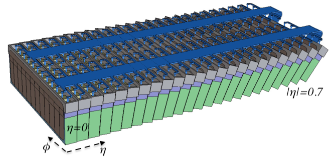 |


Figure 7
Distribution of the opening angle $\theta_{12}$ of two decay photons from $\pi^{0}$ (left) and $\eta$ (right) mesons decays as a function of the meson energy obtained at generator level from a MC simulation. The horizontal lines indicate the opening angle corresponding to a width of approximately 1, 3 and 5 cells separating the two photons. Two photons completely merge into one cluster if they fall below the one cell distance, while they start merging at a width of approximately 3 cells, depending on the clusterizer. The colored vertical lines correspond to the energy limits where two photons could still be fully resolved using the V1 (blue) and V2 (red) clusterizers. | 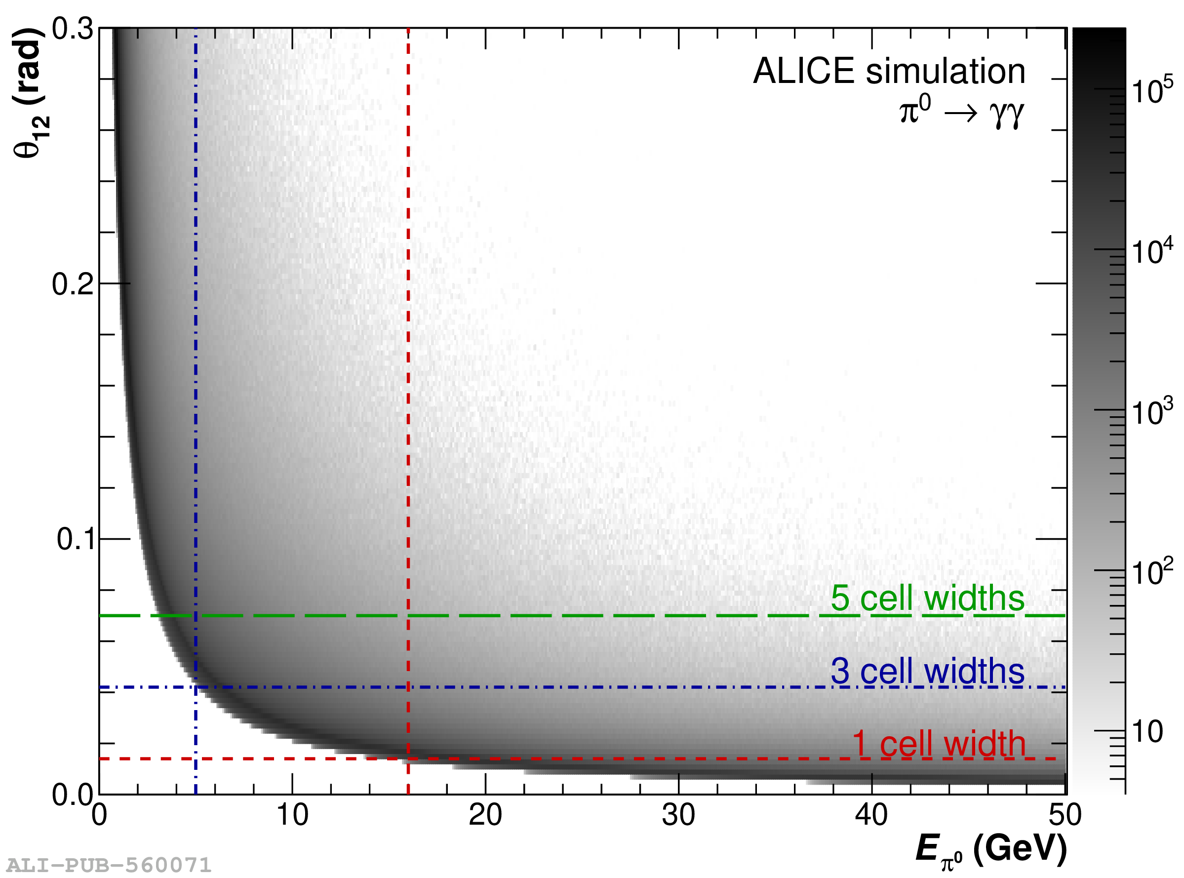 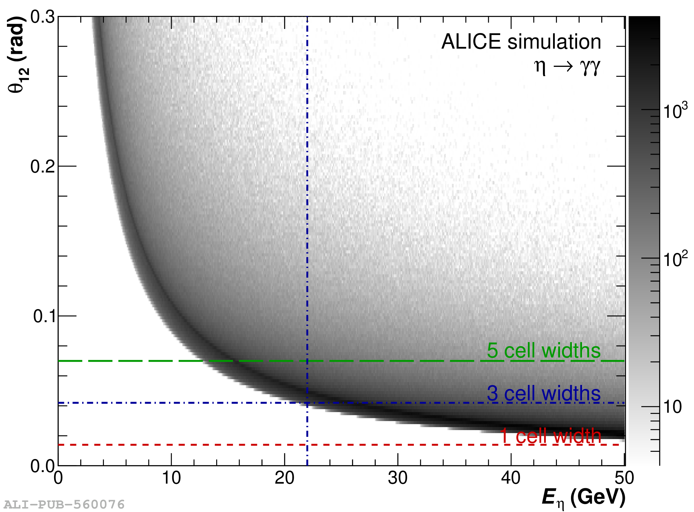 |
Figure 8
Schematic comparison of different clusterization algorithms. Only one dimension is shown for simplicity Yellow boxes represent the energy in each cell. $E_\mathrm{agg}$ is the clusterization threshold as defined in the text. The different clusters are indicated by blue and red hatched areas Each panel represents a clusterization algorithm: a) V1, b) $3 \times 3$, c) V2, d) V1+unfolding. | 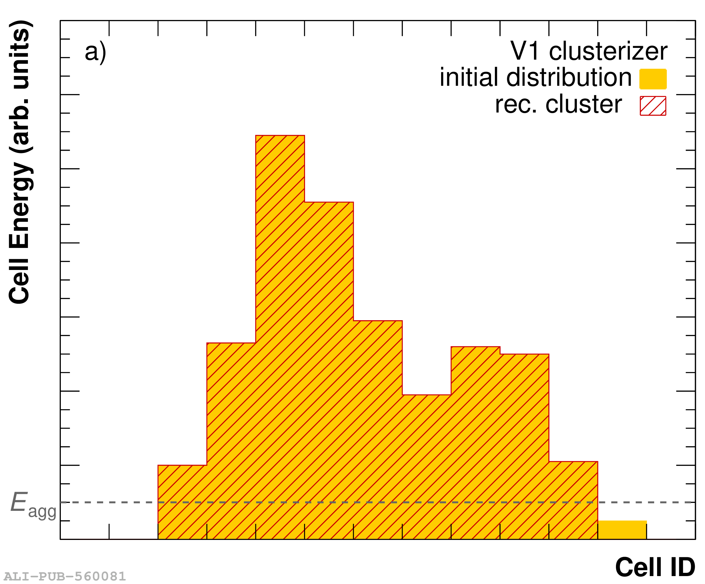 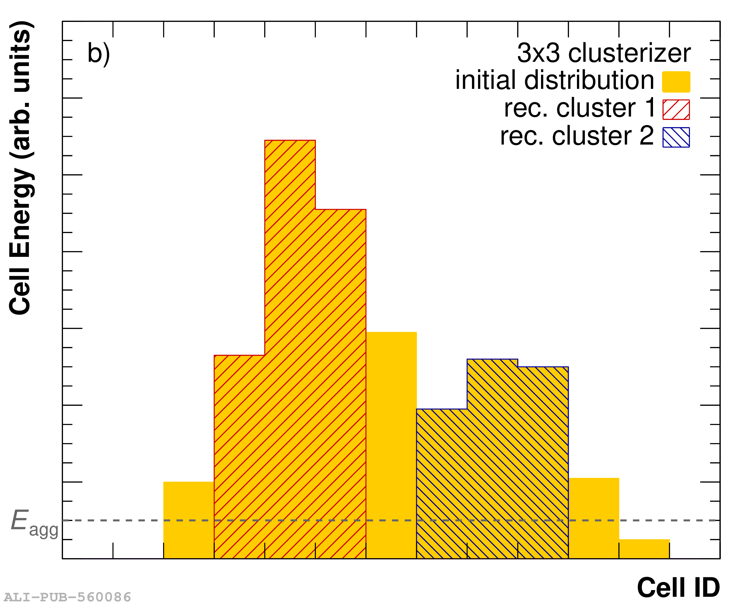 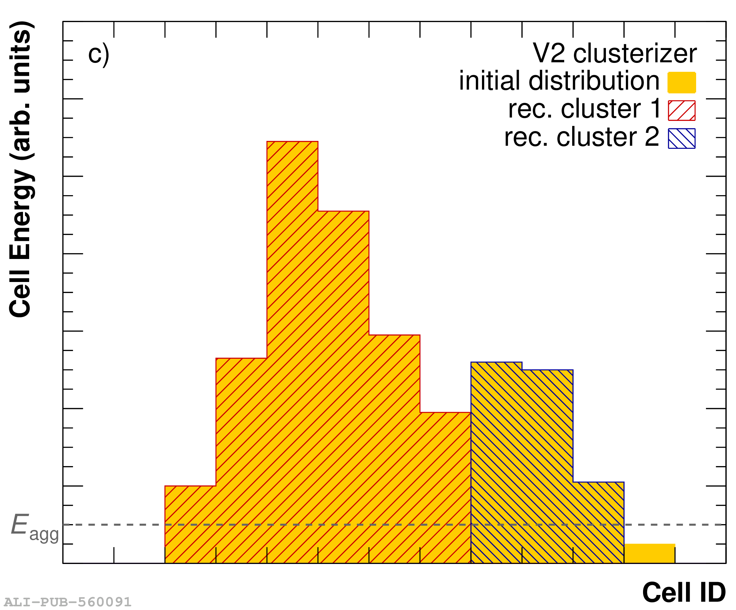 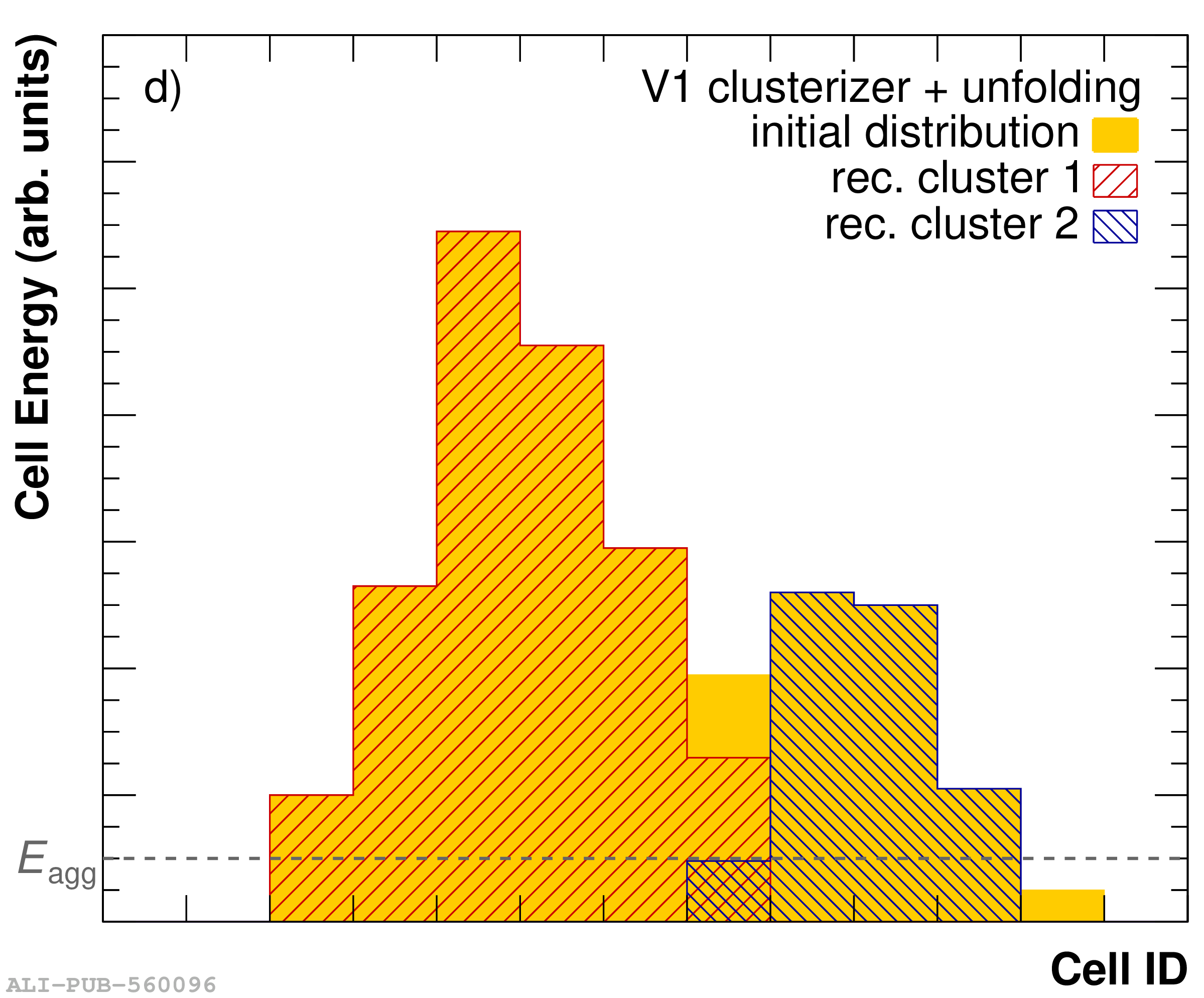 |
Figure 9
Invariant mass distribution of cluster pairs in pp collisions at $\sqrt{s}=13$ TeV for different intervals of pair energy. The differently colored lines correspond to different clusterizer types, using the same aggregation $E_\mathrm{agg}=100$ MeV and seed $E_\mathrm{seed} = 500$ MeV thresholds. The lowest bin in energy uses the data sample with minimum bias trigger, while the others are obtained from the EMCal L1 triggered data with thresholds at about $E \approx 4$ and $9$ GeV, respectively. | 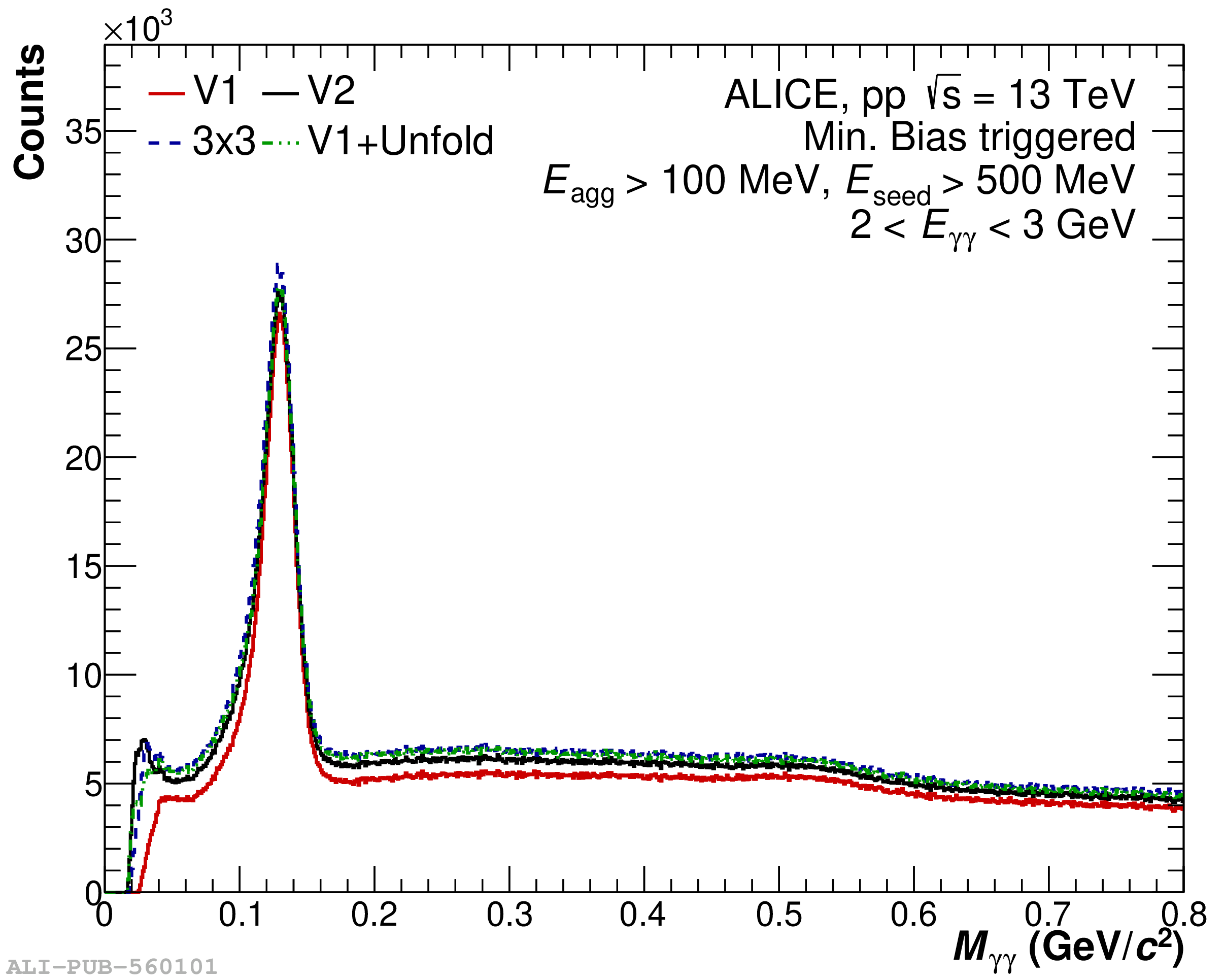 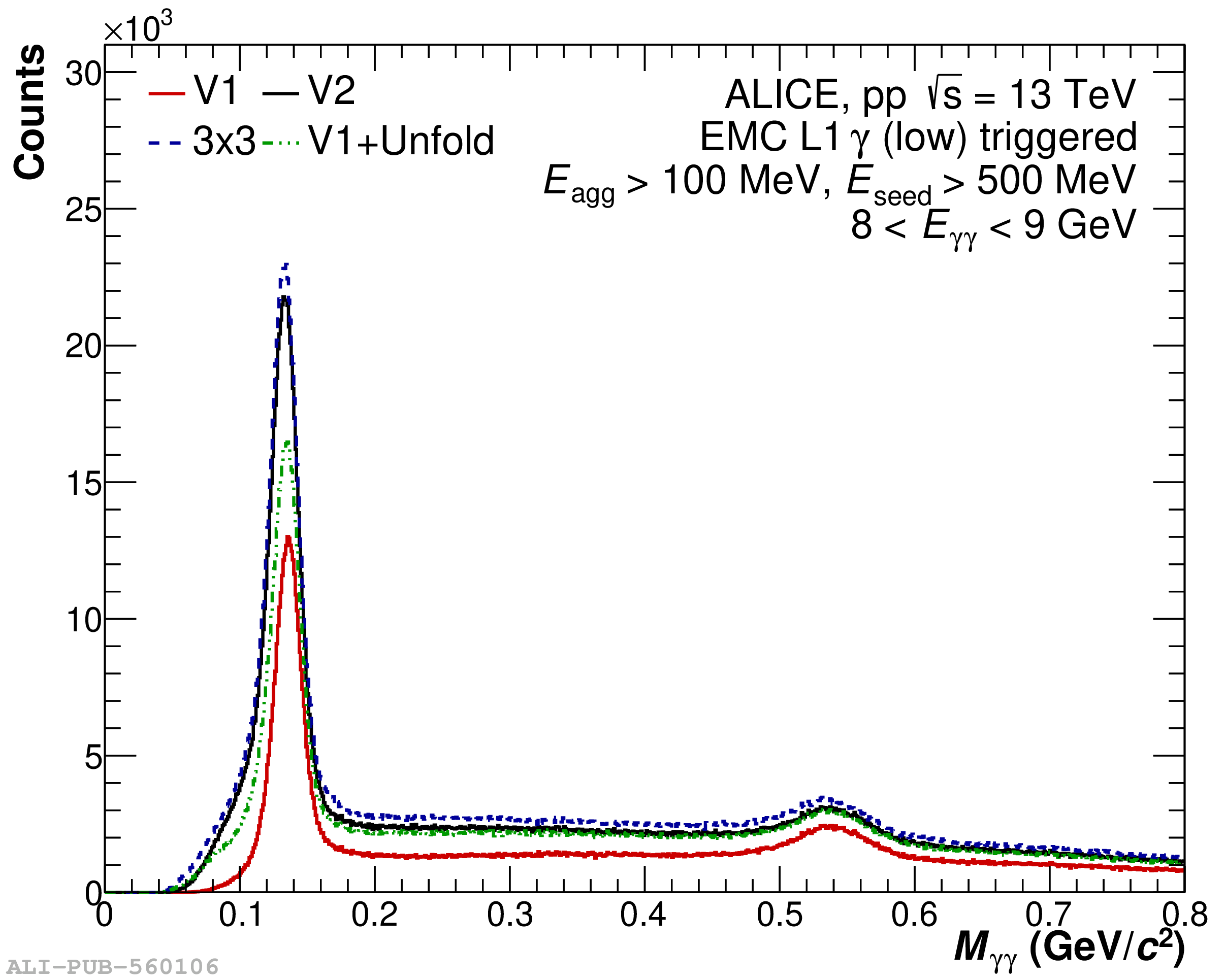 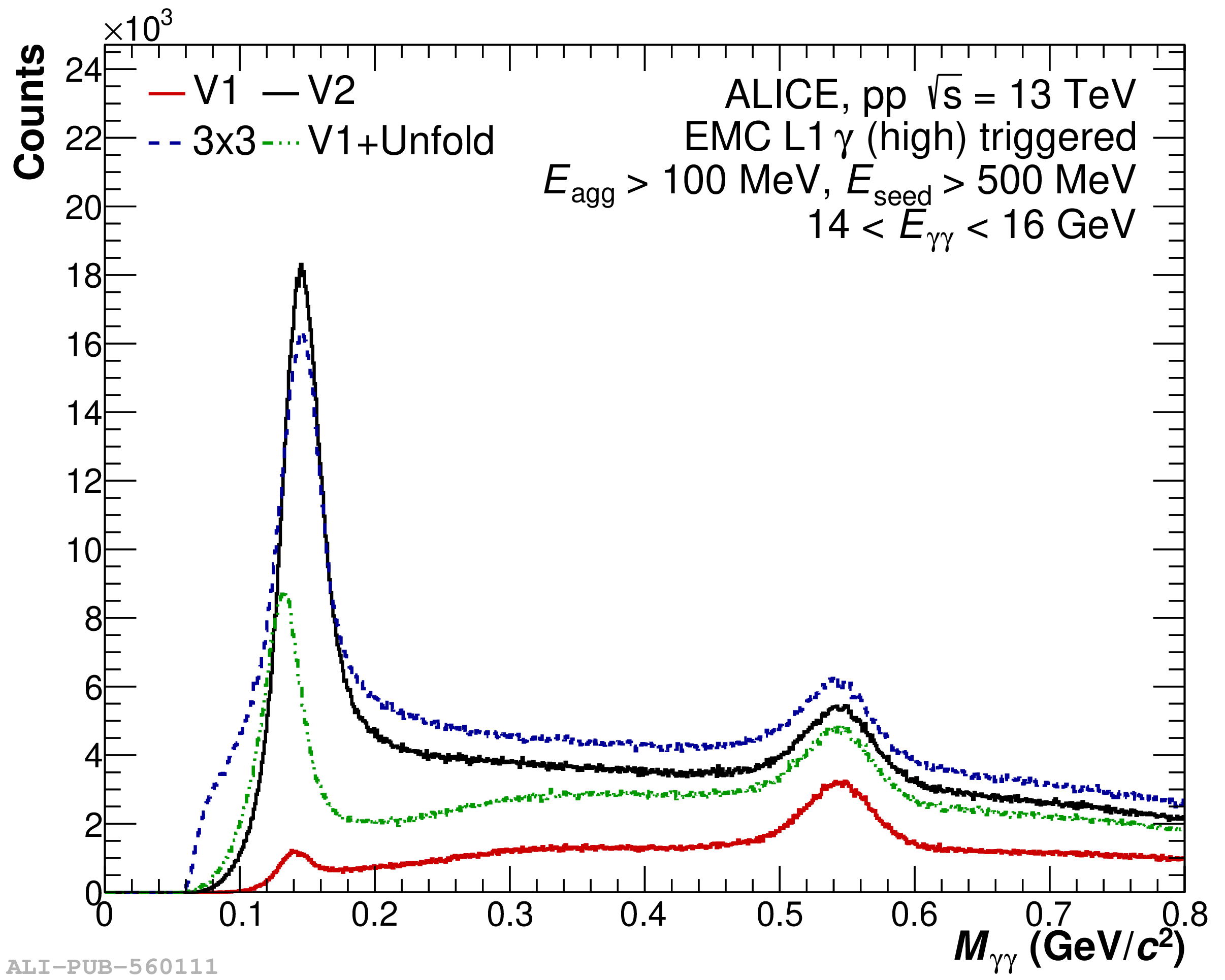 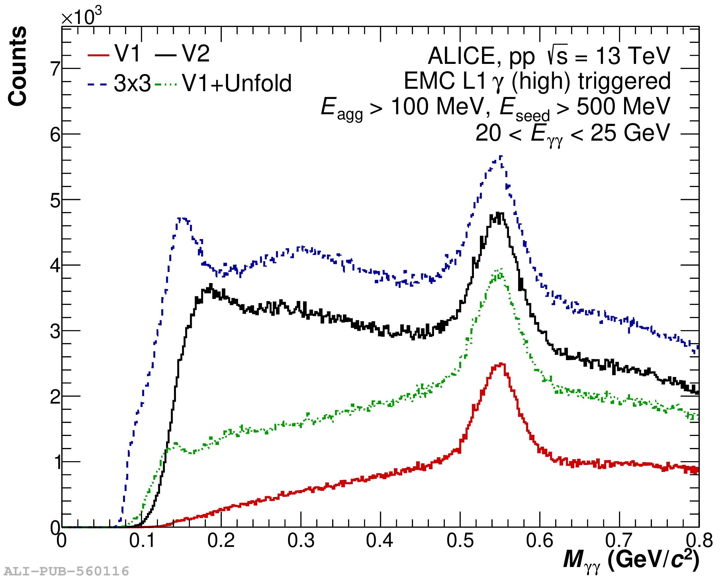 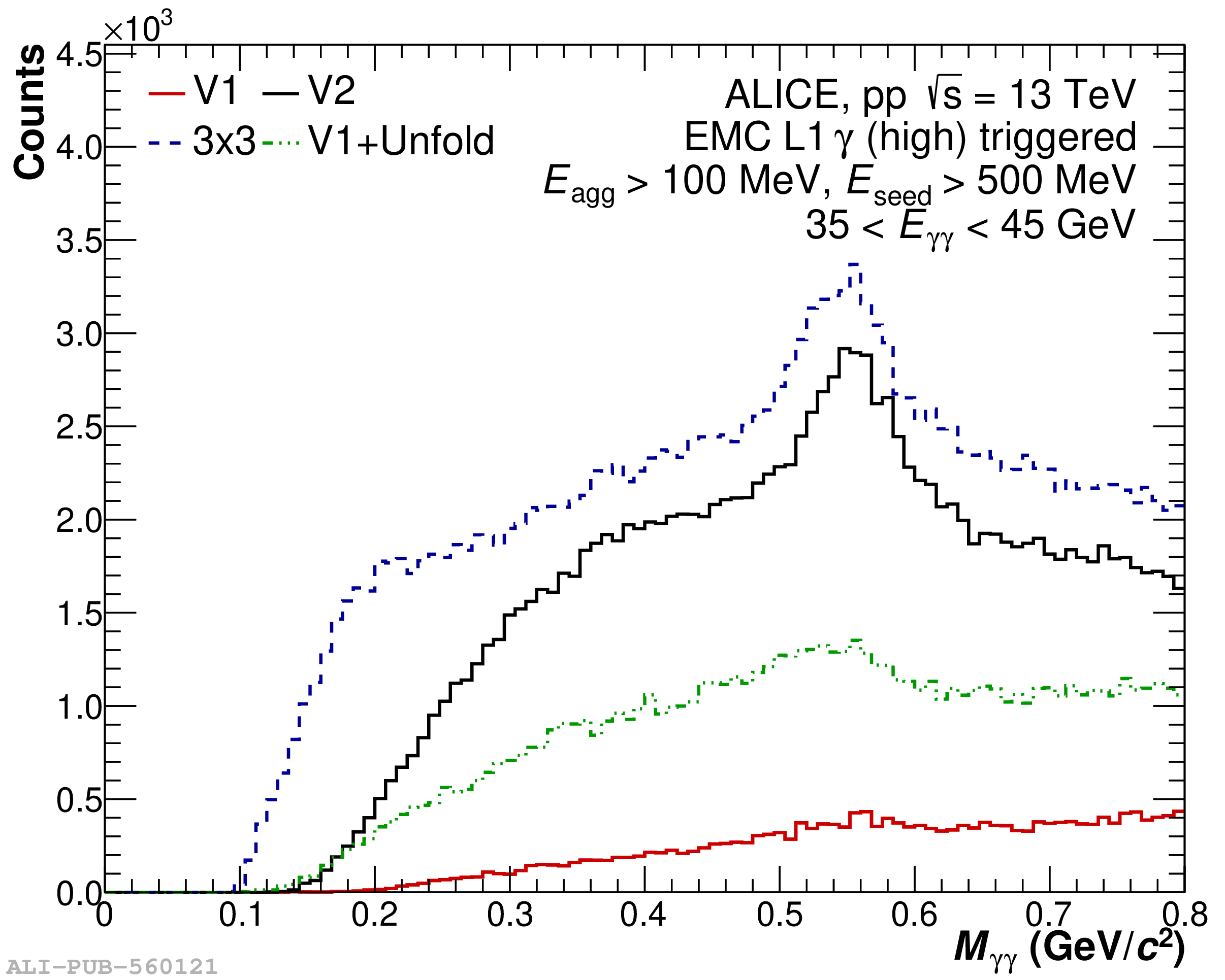 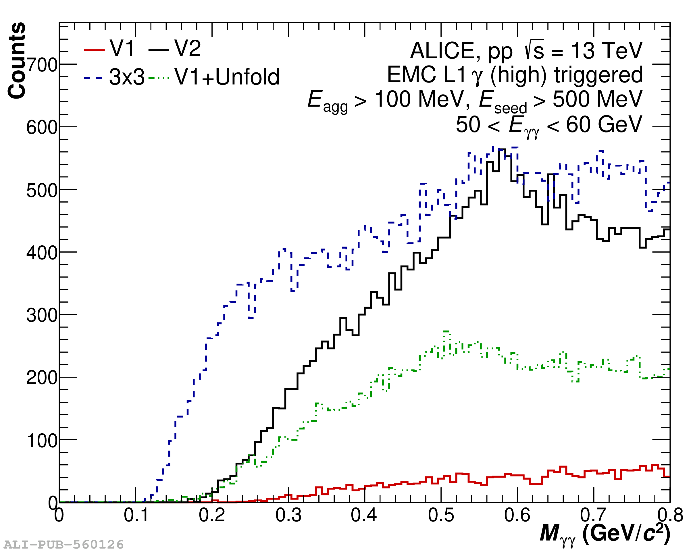 |
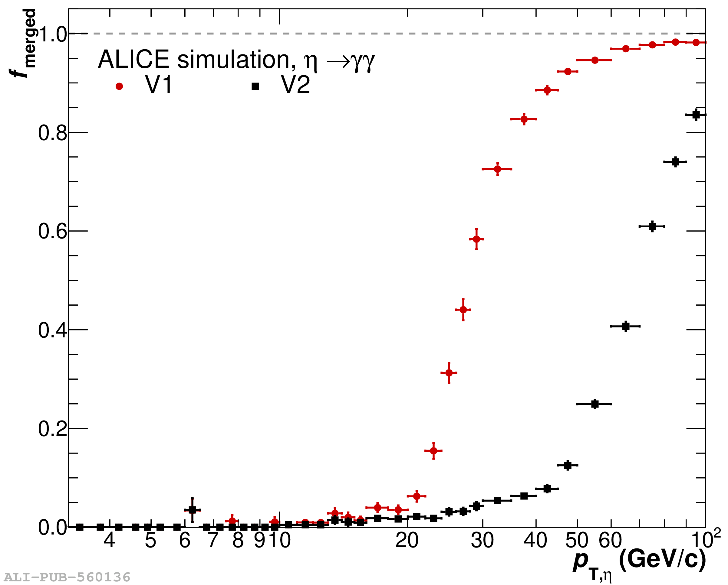
Figure 11
Distance between a cluster and the closest projected track in $\eta$ (left) or $\varphi$ angle (middle) versus the track momentum and for matched track-cluster pairs (right) in pp collisions at $\sqrt{s}=13$ TeV collected with the minimum bias trigger. Clusters are reconstructed using the V2 clusterizer. The black lines in the left and middle panels indicate the suggested selection criteria expressed in Eq. 12. | 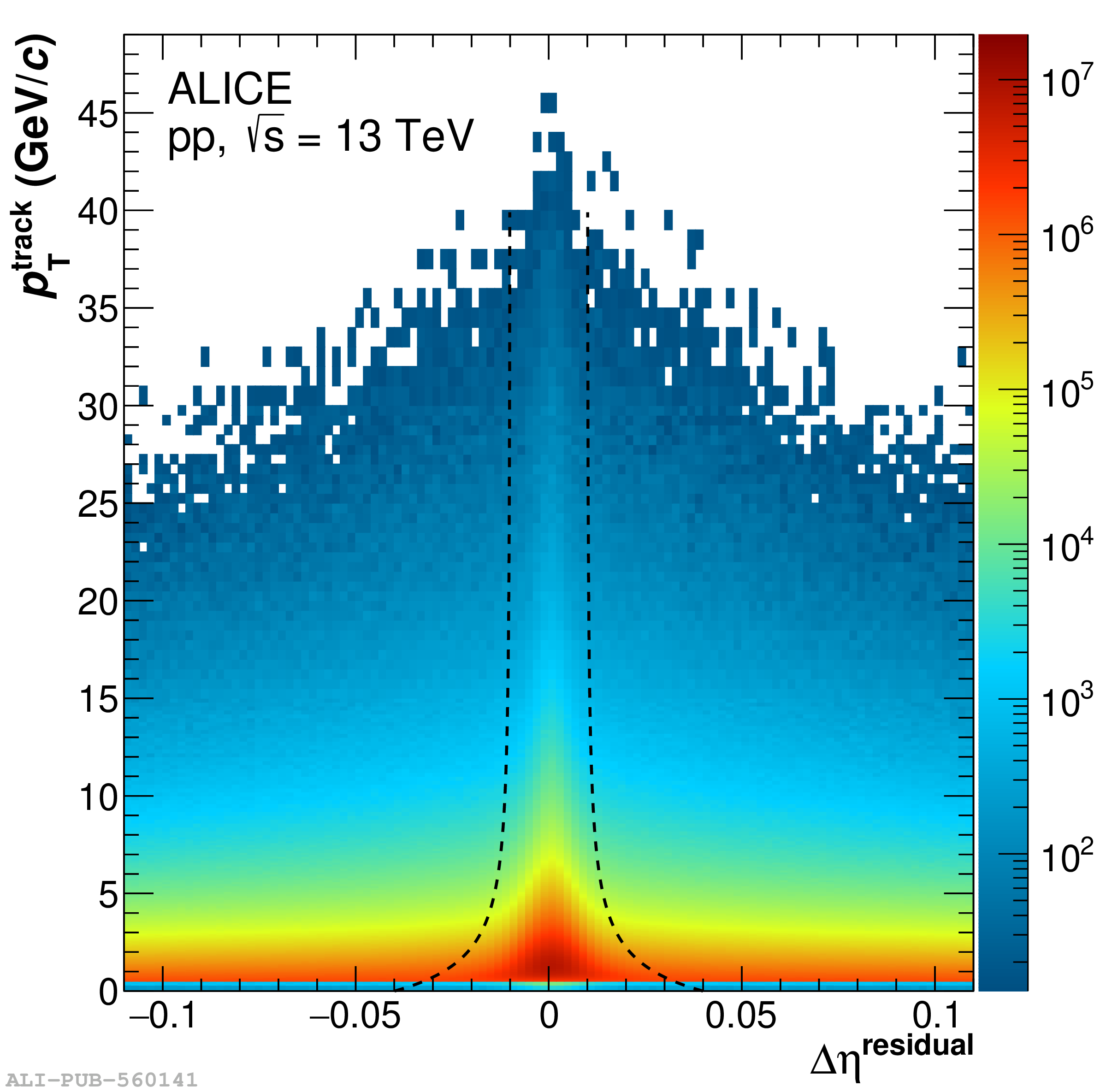 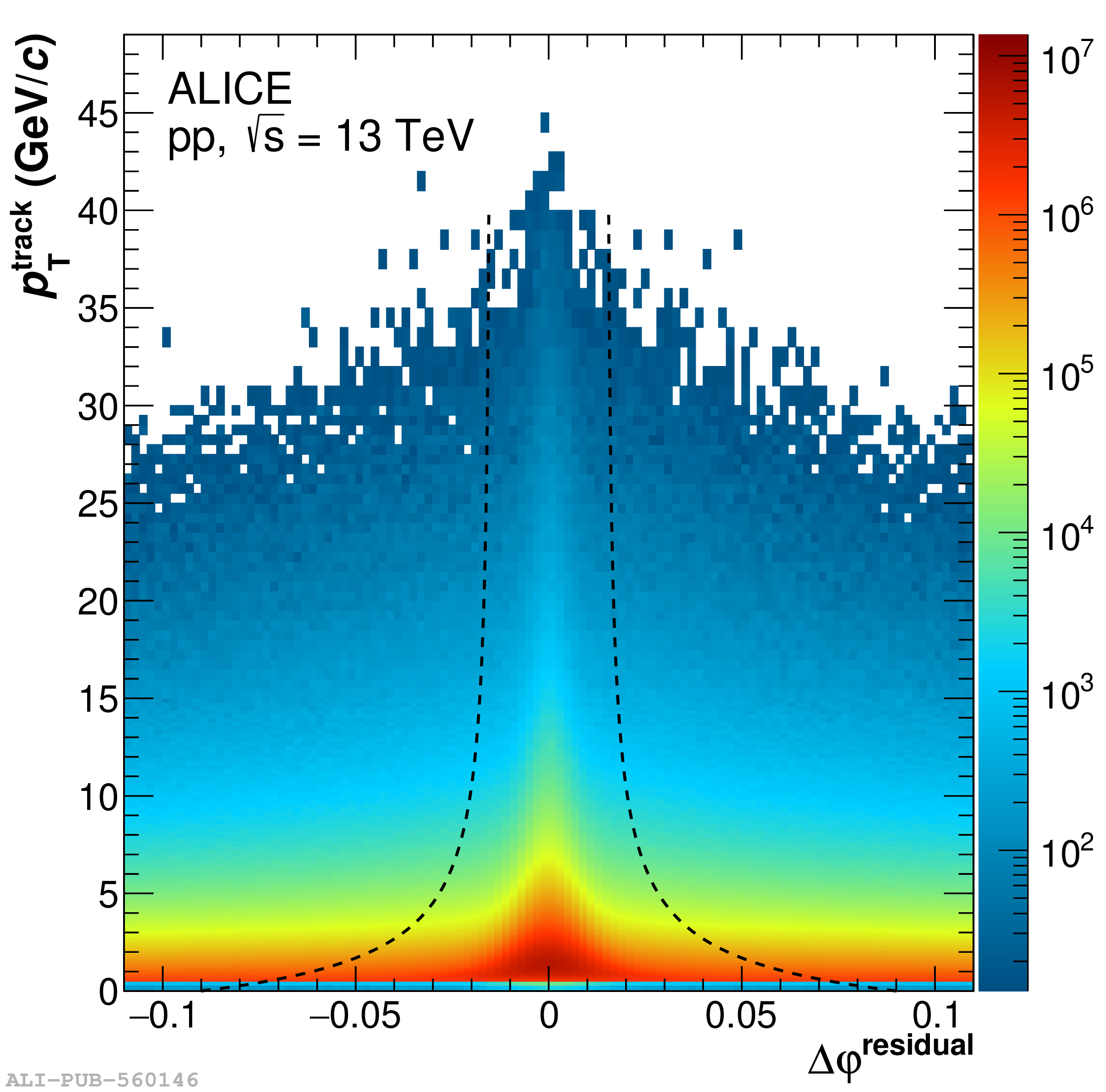  |
Figure 12
Left: cluster-veto efficiency for primary particles (dark blue open circles) and electrons (green squares) as well as conversion electrons with a production vertex below 180 cm (green closed diamonds) and above 180 cm (green open diamonds) and other secondary particles (cyan open circles) as obtained from simulations of pp collisions at $\sqrt{s}=13$ TeV. Right: fraction of fake track-to-cluster matches for clusters originating from photons (yellow open squares) and other neutral particles (red open circles). Additionally, the same categories are shown for clusters that have additional charged particle contributions for photon clusters (orange squares) and other neutral particles (light red circles). |  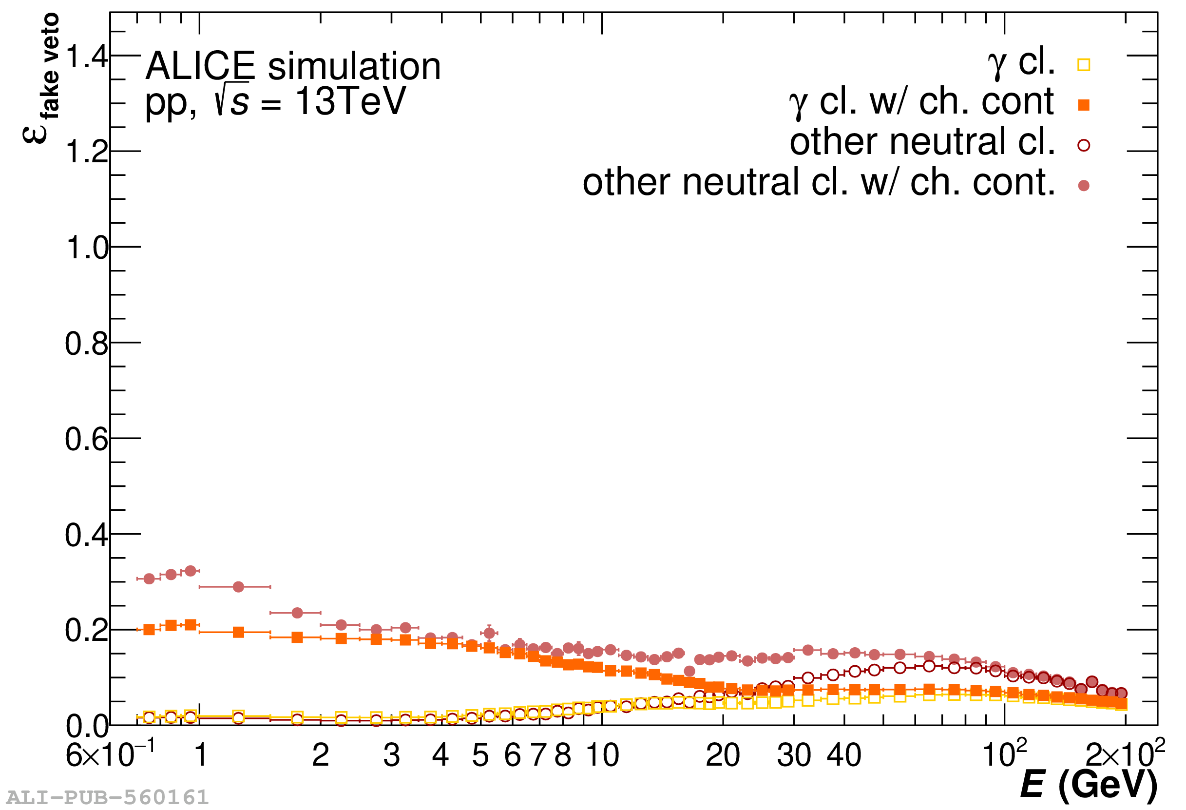 |
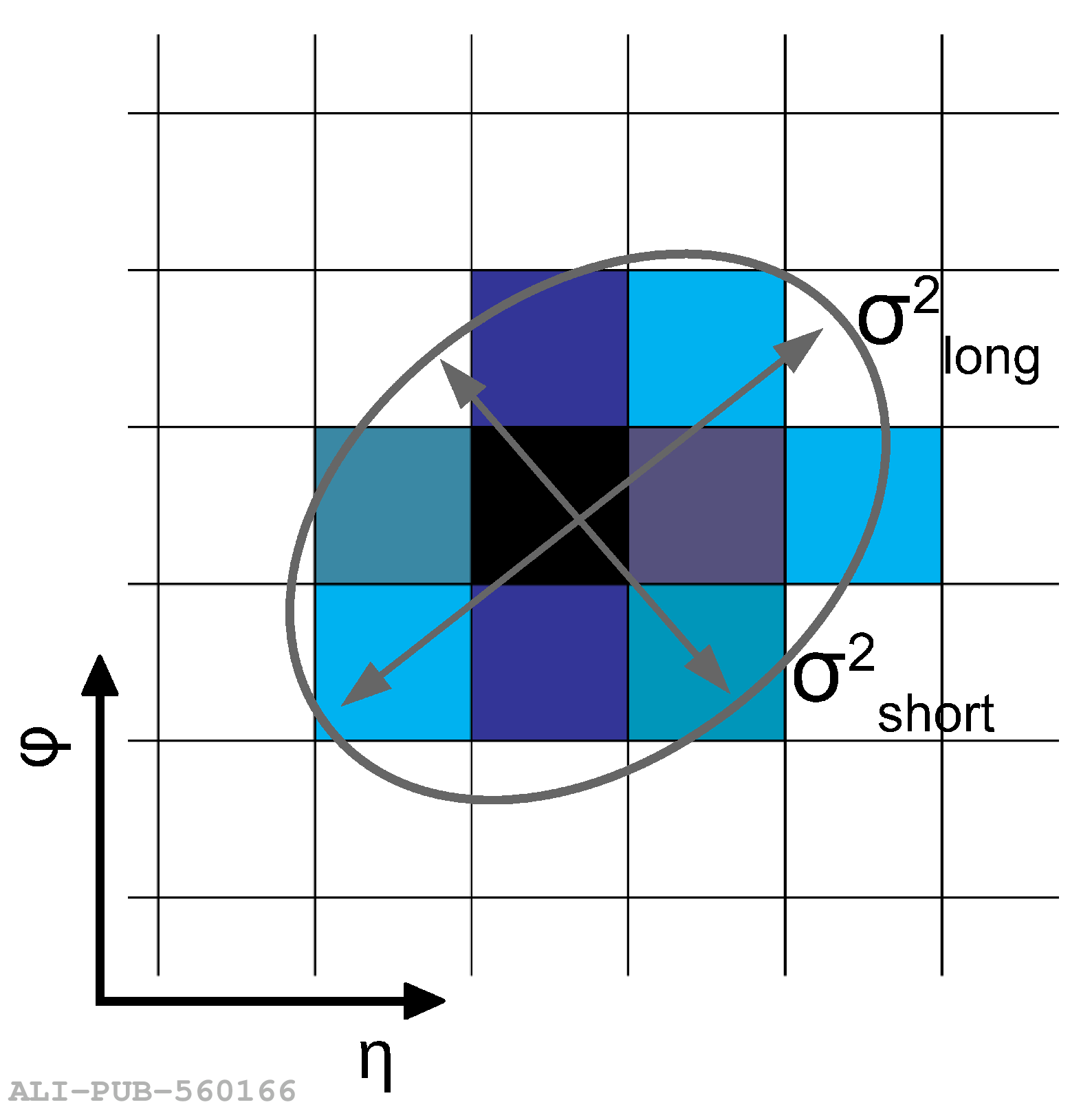
Figure 14
$\sigma_{\rm long}^{2}$ (left) and $\sigma_{\rm short}^{2}$ (right) distributions in three energy intervals for photons, electrons, hadrons, $\pi^{0}$ and $\eta$ mesons. The distributions are obtained using the V1 clusterizer from a simulation of pp collisions at $\sqrt{s}=13$ TeV performed with the PYTHIA event generator, in which events are required to contain either two jets or a jet and a high-energy direct photon. Each distribution is normalized to its integral. A model simulating the effect of the cross talk was applied as discussed in Sec. 5.8. | 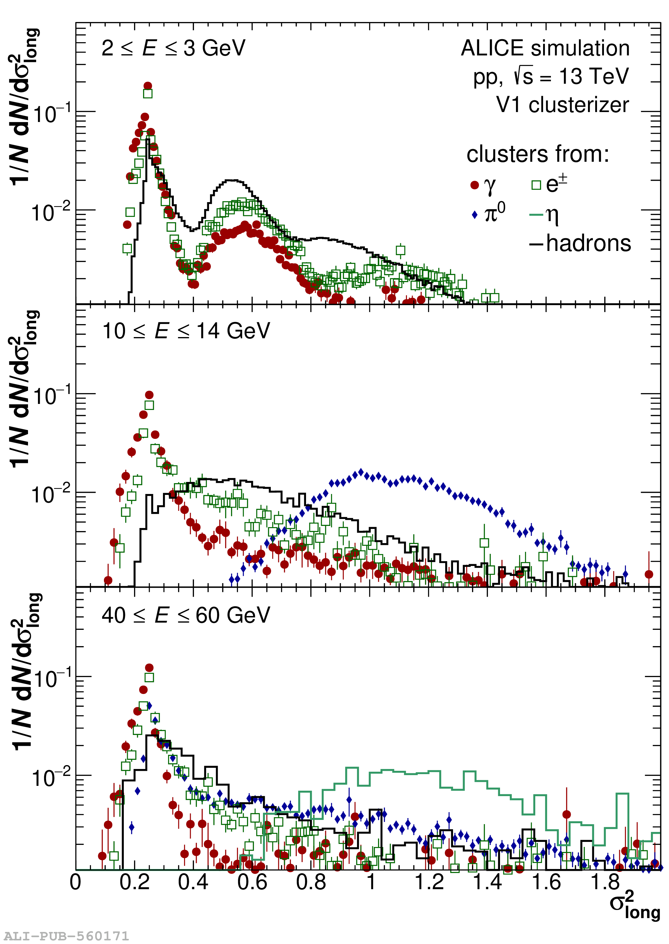  |
Figure 15
Distributions of $\sigma_{\rm long}^{2}$ versus cluster energy in pp collisions at $\sqrt{s}=13$ TeV triggered by the EMCal L1 at approximately 9 GeV for the V2 (left) and V1 clusterizer (right). Each energy bin is normalized to its integral and exotic clusters were rejected (Sec. 3.4.3). |   |
Figure 16
Left: number of cells as a function of the cluster energy found with the V2 clusterizer in pp collisions at $\sqrt{s}=13$ TeV using the EMCal high threshold L1 $\gamma$ trigger. The region below the lines is populated by exotic clusters. The distribution for each energy bin is normalized to its integral. Right: comparison of $n_{\text{cells}}$ probability distributions for measured data (black), projection of the left plot, to simulated (blue) collisions for two different cluster energy bins. Each distribution is normalized by the integral of the distribution for $n_{\rm cells}>10$. | 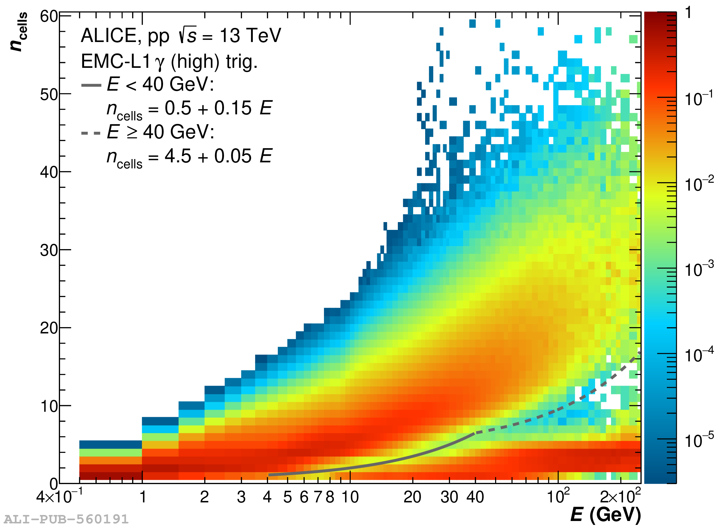 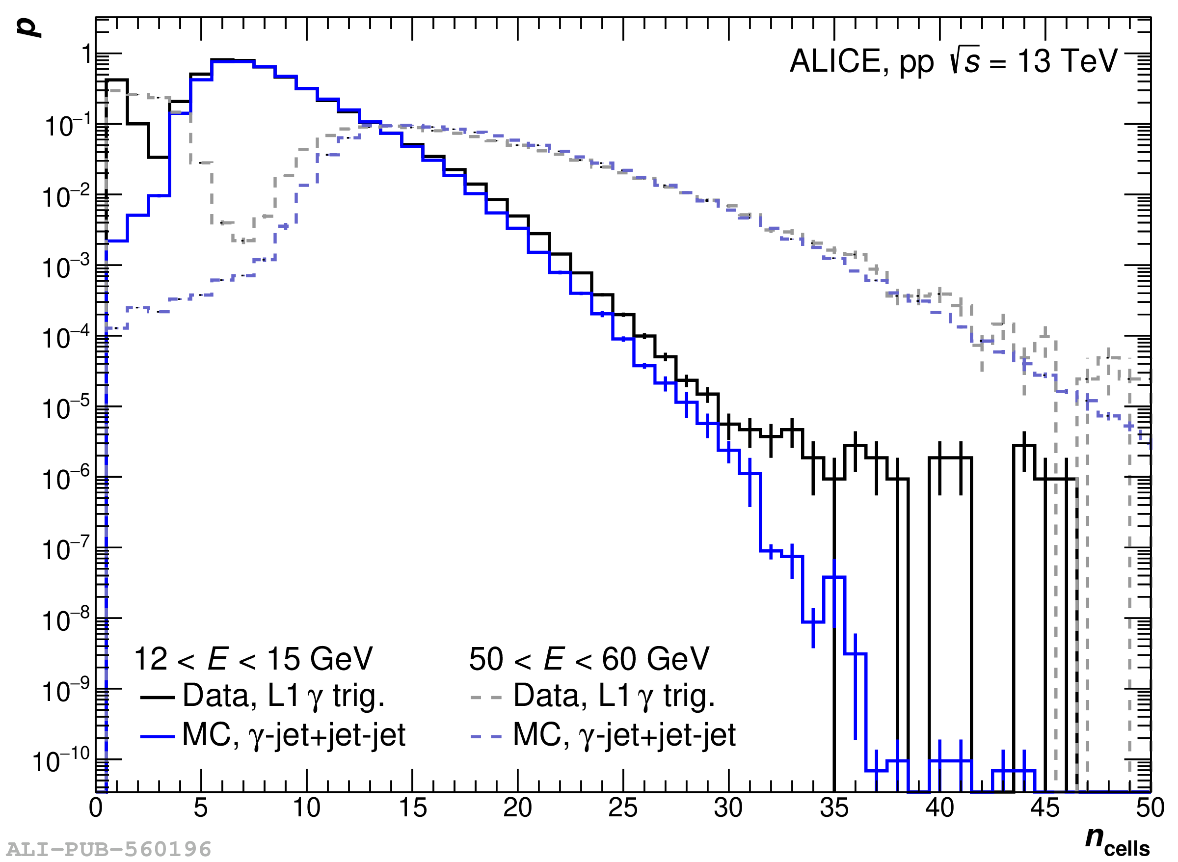 |
Figure 17
Left: "exoticity" ($F_{\rm +}$) as function of the cluster energy found with the V2 clusterizer in pp collisions at $\sqrt{s}=13$ TeV using the EMCal high threshold L1 $\gamma$ trigger. The region above the line is populated by exotic clusters. The distributions are normalized to have an integral of unity for each energy bin. Right: comparison of $F_{+}$ probability distributions for measured data (black), projection of the left panel, and simulated (blue) collisions for two different cluster-energy intervals. Each distribution is normalized by the integral of the distribution for $F_{+}< 0.85$. |  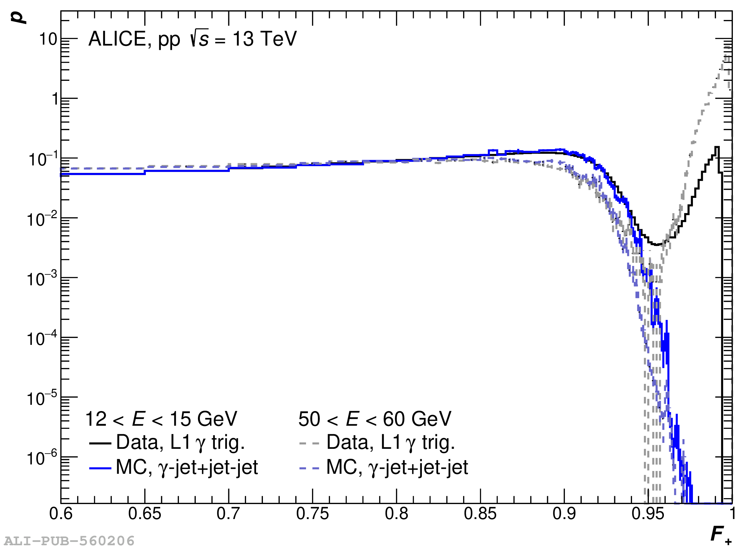 |
Figure 18
Left: cluster time for exotic ($F_{+}>$ 0.97 and non-exotic ($F_{+}< $ 0.97) clusters. The additional peaks in the time distribution beyond $100$ ns arise from additional bunch crossings, which could not be rejected by the online Past-Future protection using the V0 detector. Right: difference in time of the most and second most energetic cell in the cluster for exotic and non exotic clusters. Both distributions are obtained for V2 clusters with energy in the interval $8 < E < 10$ GeV from data taken from pp collisions at $\sqrt{s}=13$ TeV. |   |
Figure 19
$\sigma_{\rm long}^{2}$ as a function of the exoticity parameter $F_{+}$ obtained from V2 clusters with $12< E< 15$ GeV. The distributions are shown for pp collisions at $\sqrt{s}=13$ TeV using the EMCal L1 $\gamma$ (high) trigger at $E^{\rm L1-trig}=9$ GeV (left) and Pb$-$Pb collisions at $\sqrt{s_{\rm NN}}=5.02$ TeV for $0-10$% central collisions. |  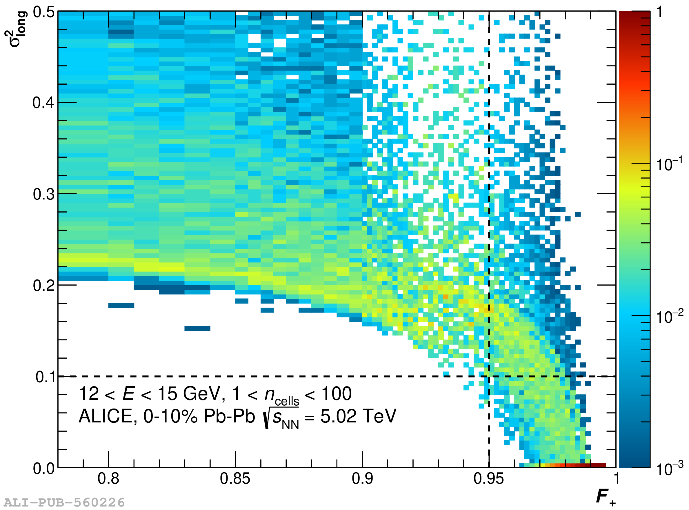 |

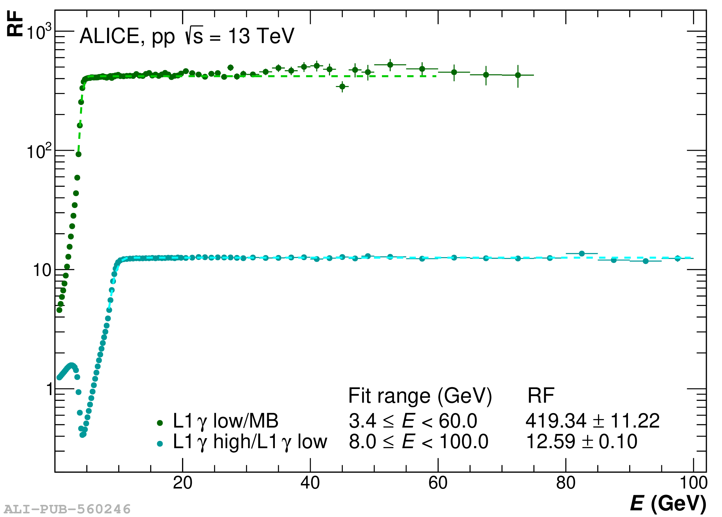
Figure 24
Left: trigger rejection of the jet triggers obtained from calorimeter-based jets with $R$ = 0.2 in pp collisions at $\sqrt{s}=13$ TeV collected in 2017 and 2018. Ratios are with respect to minimum-bias events (red) or to events triggered by the low-threshold jet trigger (yellow). Right: corresponding trigger efficiency of the jet triggers in pp collisions at $\sqrt{s}=13$ TeV obtained with fast simulations on cell level and with full simulations including the trigger response. | 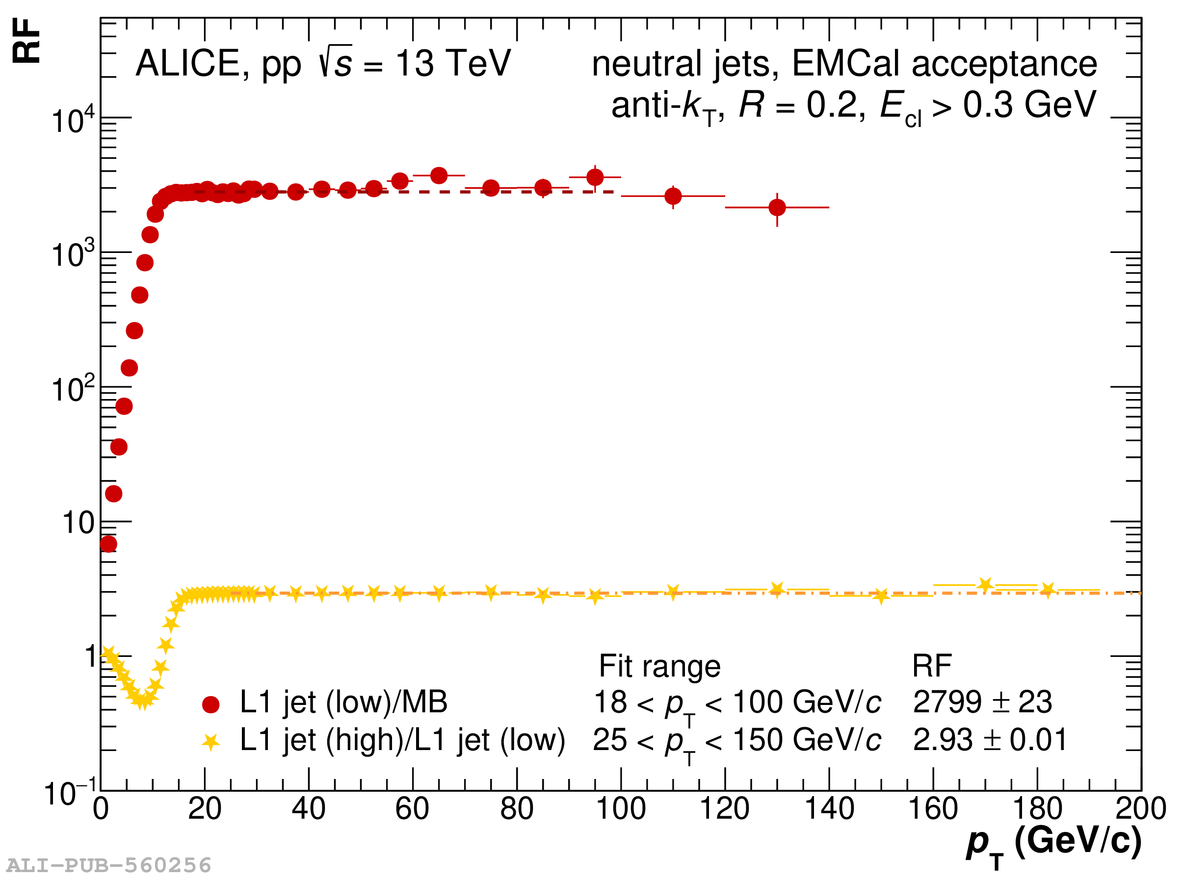 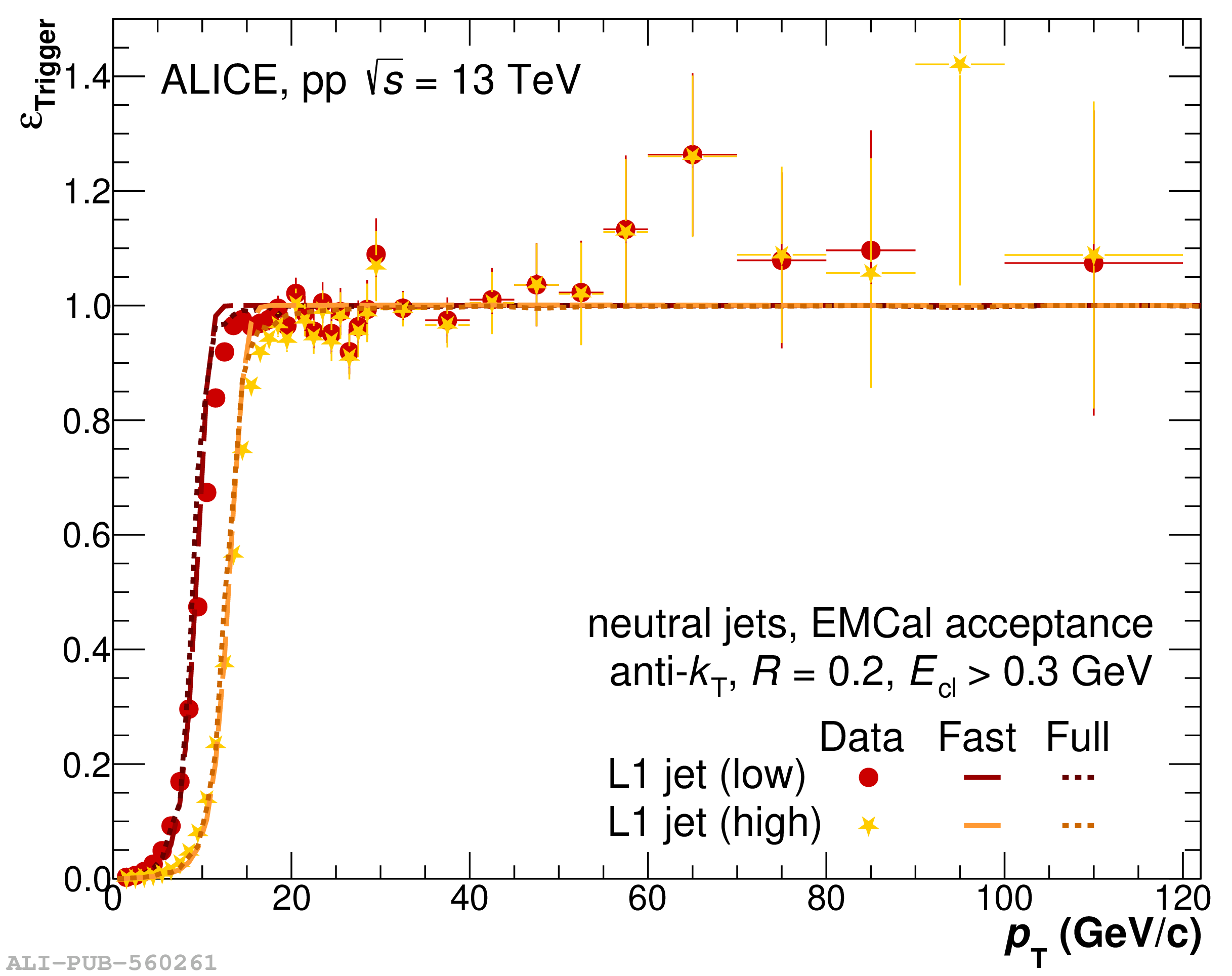 |
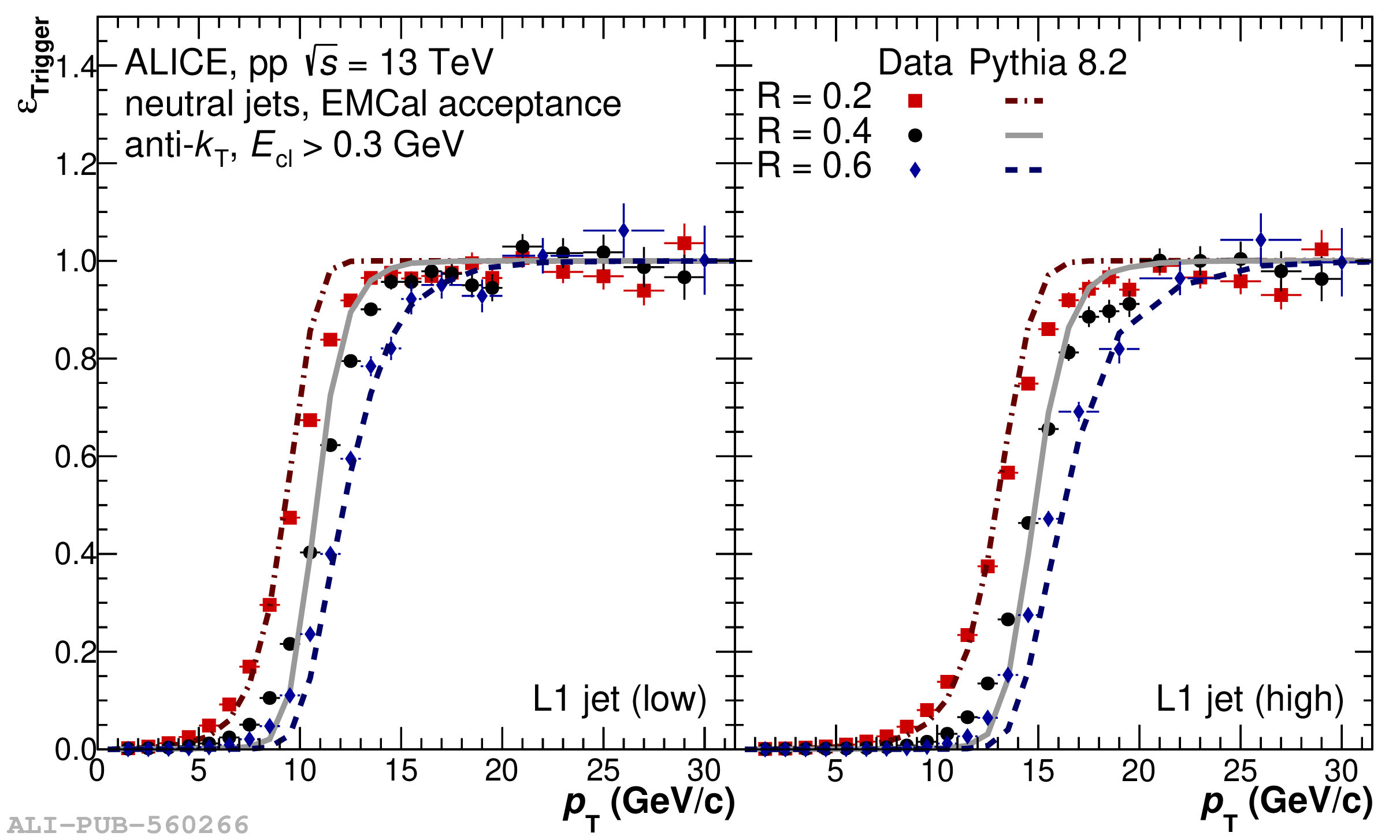
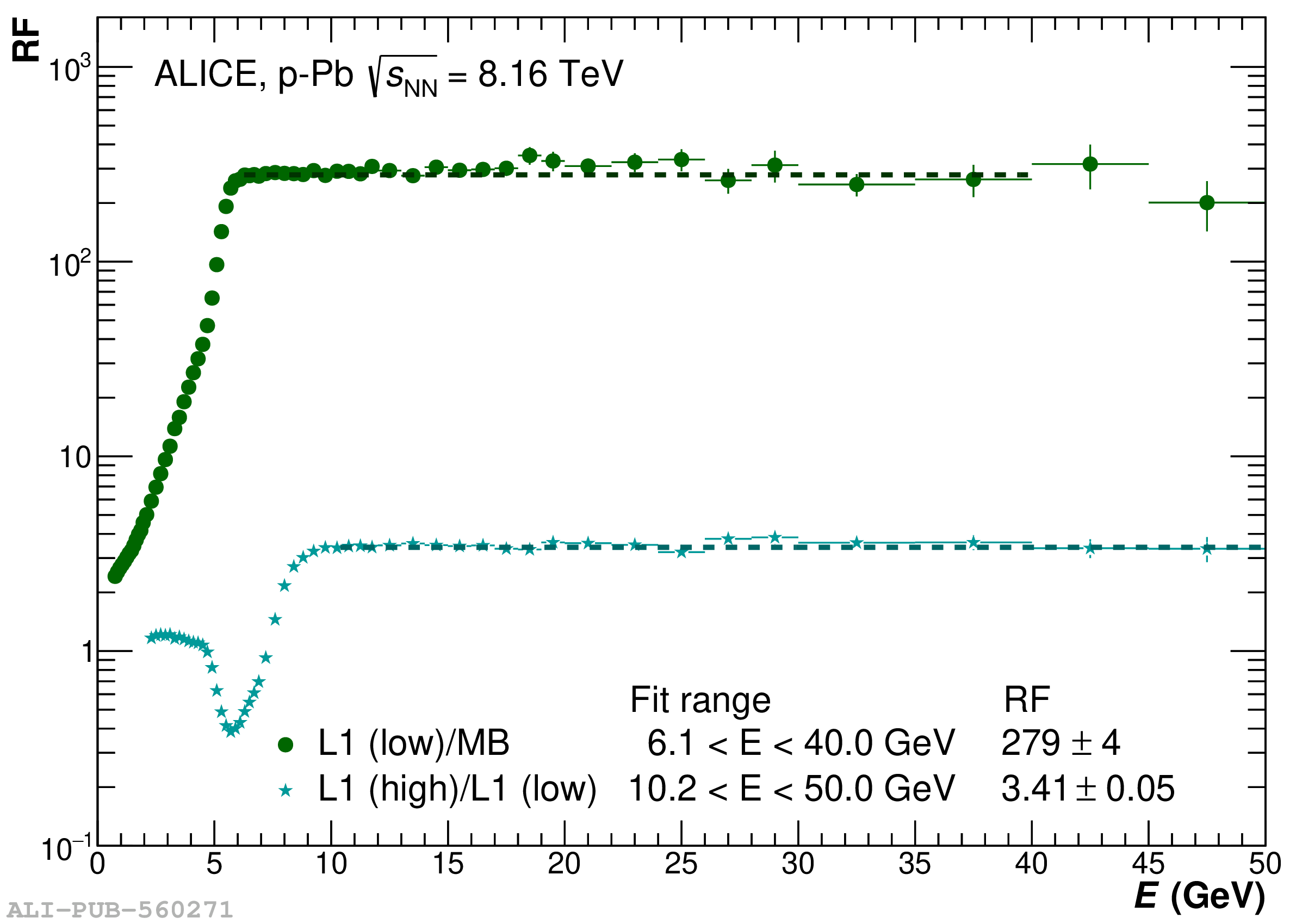

Figure 28
Left: Centrality percentile distribution of EMCal L1 $\gamma$ triggered events (red) in comparison to the pure minimum bias distribution and minimum bias triggered events with a 10 GeV cluster in the event. Right: Trigger RF for the EMCal or DCal L1 $\gamma$ triggers in different centrality classes for Pb$-$Pb collisions at $\sqrt{s_{\rm NN}}=5.02$ TeV. Only statistical uncertainties of the trigger RF are given in the legend. | 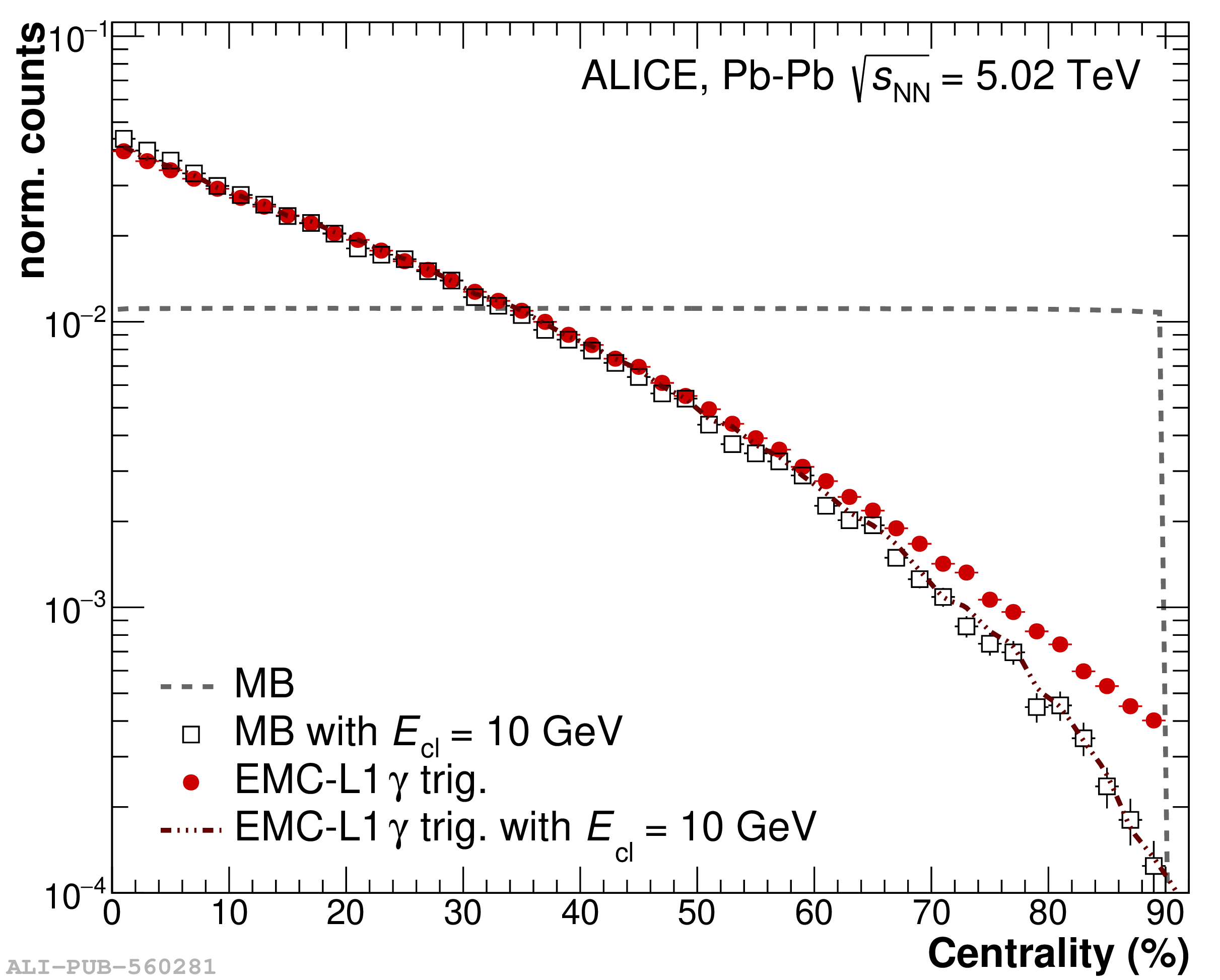  |
Figure 29
Comparison of the trigger RF based on clusters and full jets for the EMCal L1 $\gamma$ and jet trigger in 0$-$10% (left) and 50$-$90% (right) central Pb$-$Pb collisions at $\sqrt{s_{\rm NN}}=$ 5.02 TeV. Only statistical uncertainties of the trigger RF are given in the legend. | 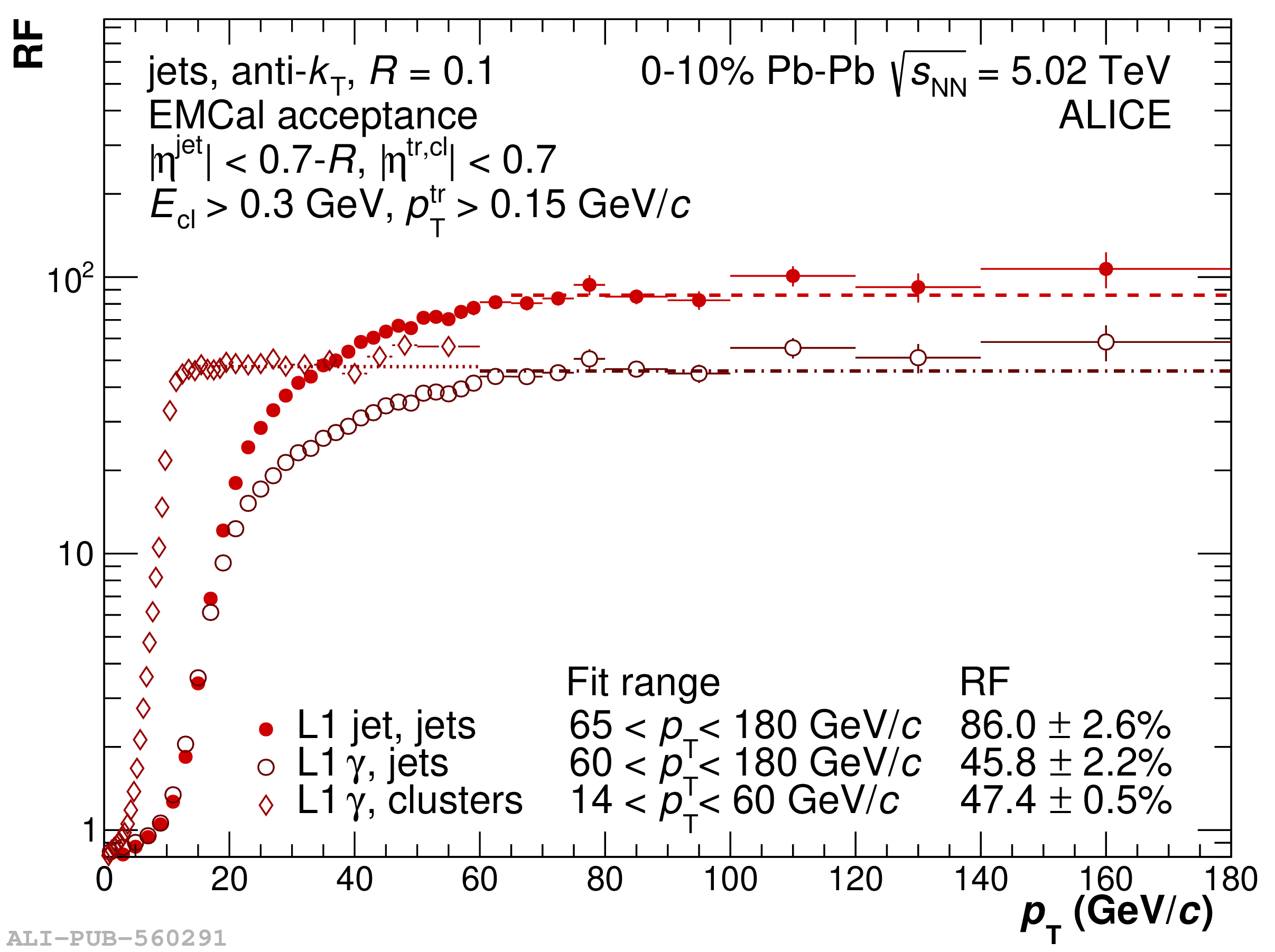 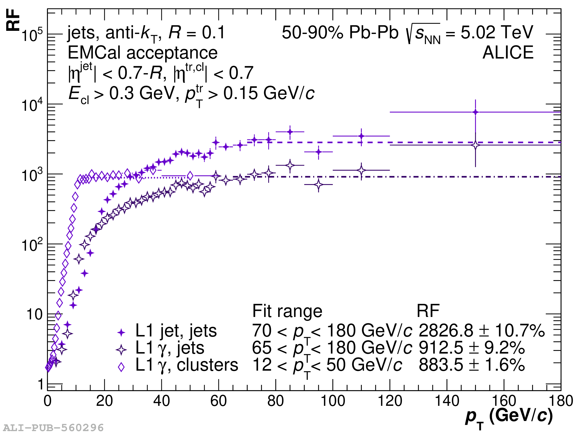 |
Figure 30
Raw distribution of the invariant mass of cluster pairs in EMCal (left) and DCal (right) for one run of 2018 data taking obtained during the QA process. The red line corresponds to a fit to the invariant mass distribution with a Gaussian function for the $\pi^{0}$ signal and a second-order polynomial for the background. The fit parameters are used to monitor the performance of the reconstruction and of the detectors. In the displayed run, 819535 events were collected. | 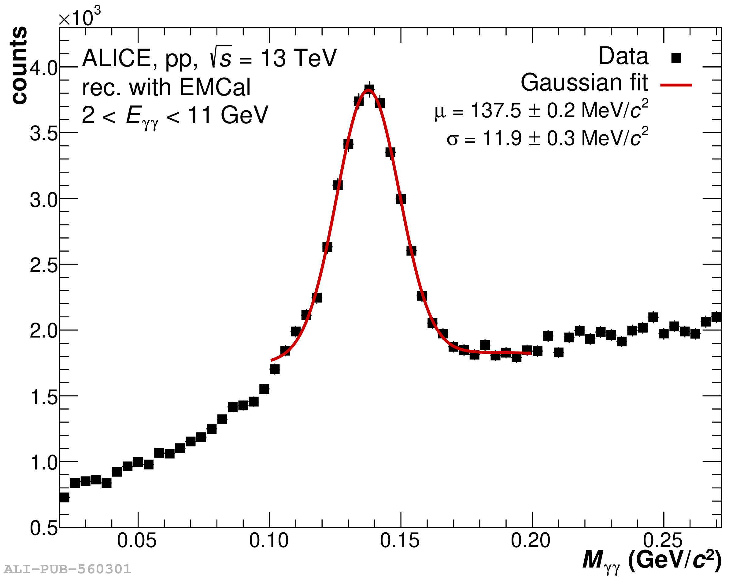 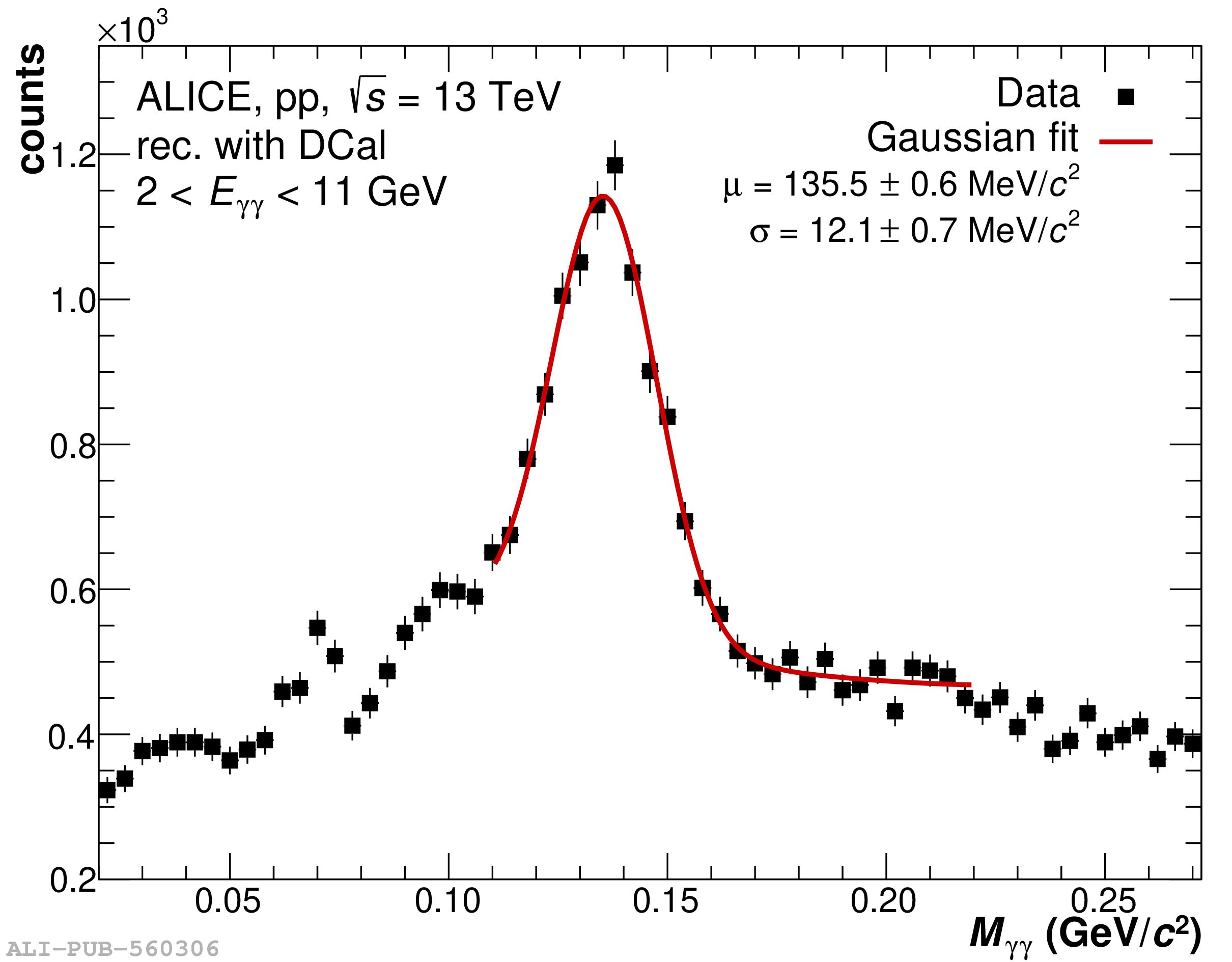 |
Figure 31
Mean number of clusters per event as a function of the run index for pp collisions at $\sqrt{s}=$ 13 TeV. Example runs with similar data-taking conditions are displayed. Only clusters with energy above 0.5 GeV were used for the mean estimation. The gray vertical lines correspond to the start of different data-taking years. | 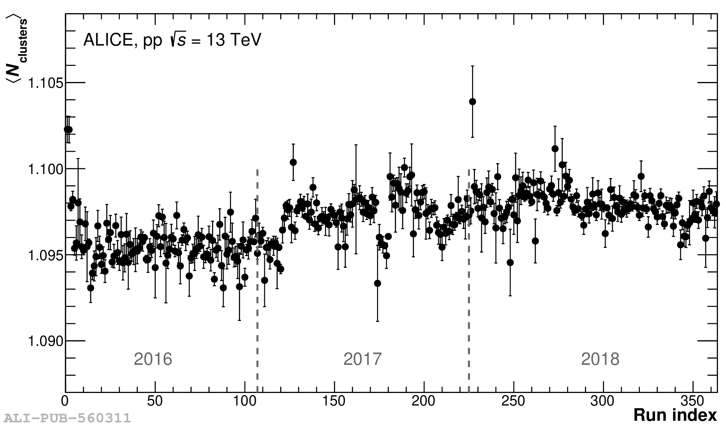 |
Figure 32
Mean number of cells per cluster (left) and mean cluster energy (right) for a selection of SM as a function of the run index in pp collisions at $\sqrt{s}=$ 13 TeV. Example runs with similar data-taking conditions are displayed. Only clusters with energy above 0.5 GeV were used for the mean estimation. The vertical red line indicates the run at which the 2 last DCal SM were inserted into the readout. The vertical gray lines correspond to the start of different data-taking years. |   |
Figure 35
Schematic view of the ALICE EMCal mini-module at the PS T10 beam line. The beam enters from the right. The Cherenkov detector was used for identification of the beam particle. The mini-module could be moved in the directions indicated by the red arrows in order to scan different towers. | 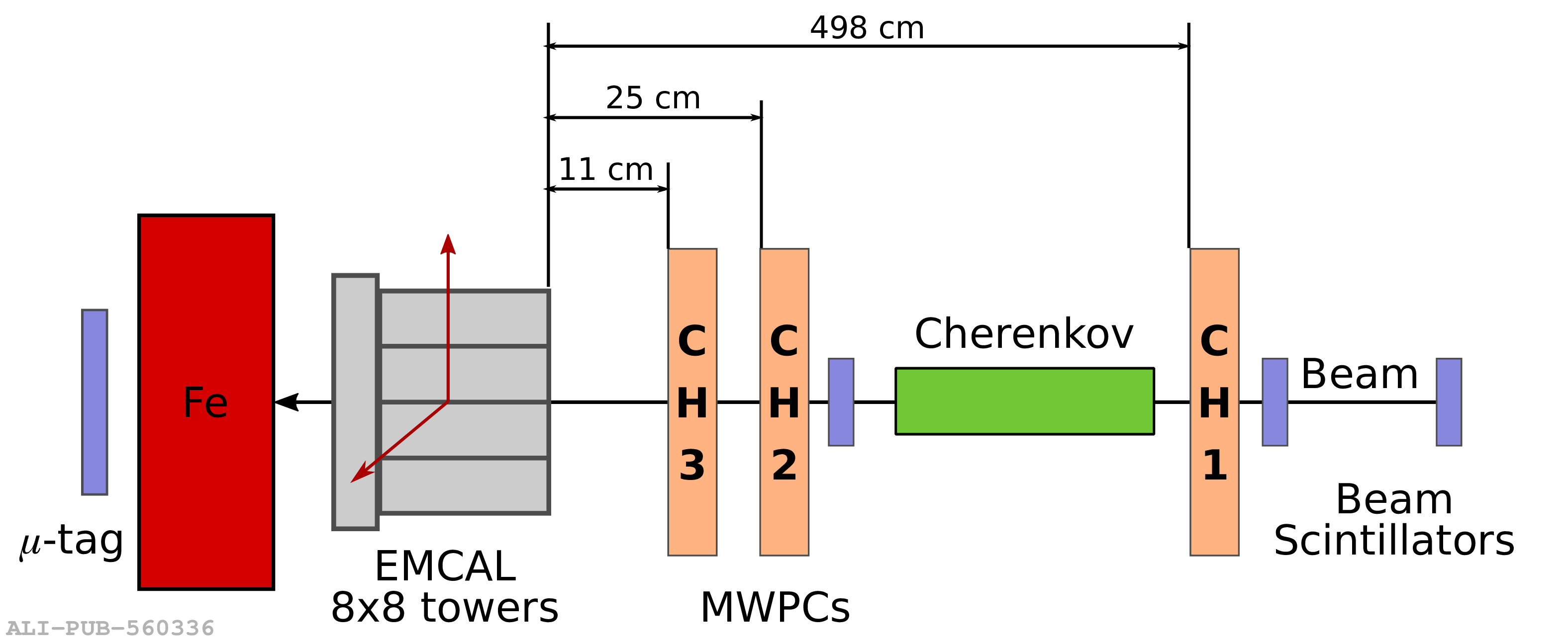 |
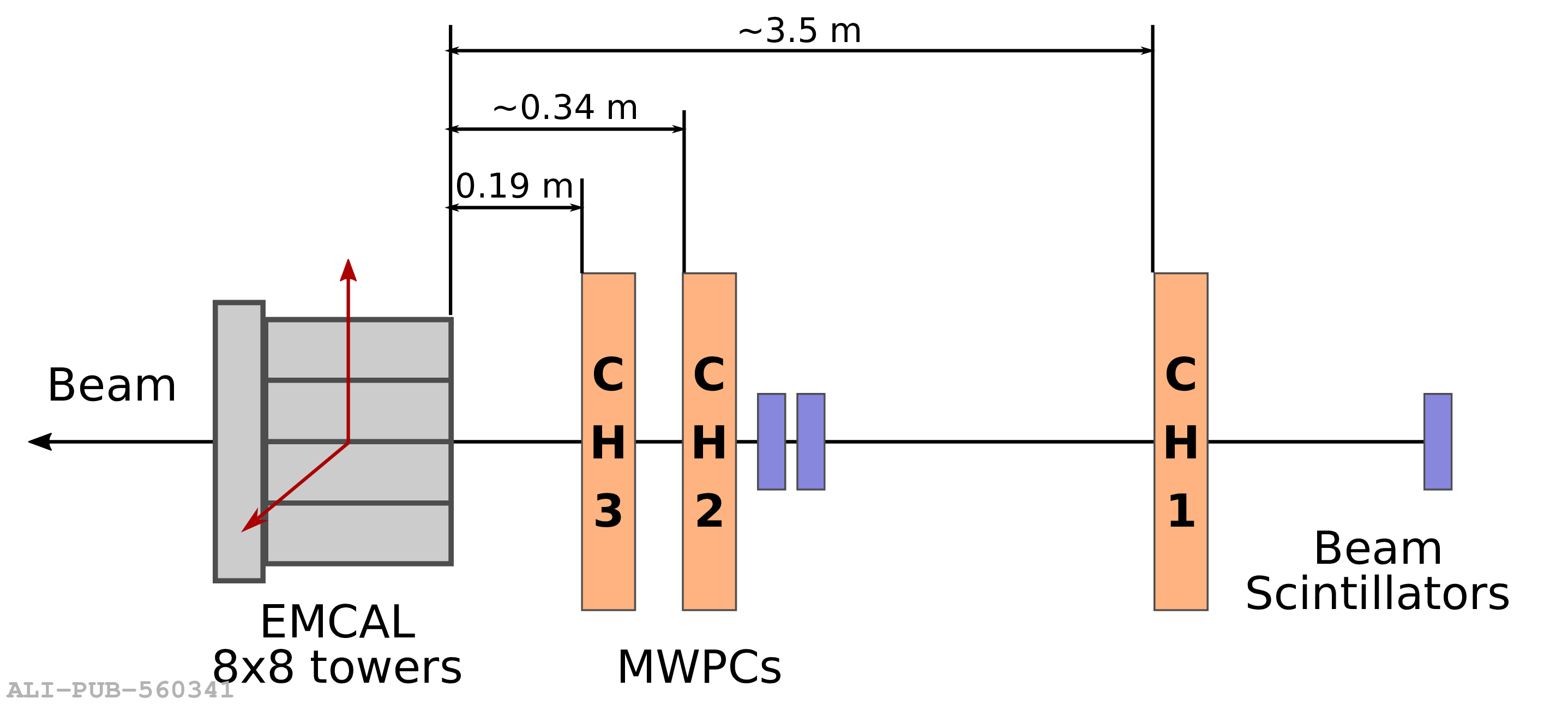
Figure 37
Left: Measured pulse amplitude ($A_{\rm out}$) as a function of input pulse amplitude obtained from laboratory measurements The dashed gray line indicates the case of a linear shaper. Right: Comparison of laboratory measurements with the Test Beam (TB) data on missing energy ($E_{\rm miss}$) as a function of the measured energy. | 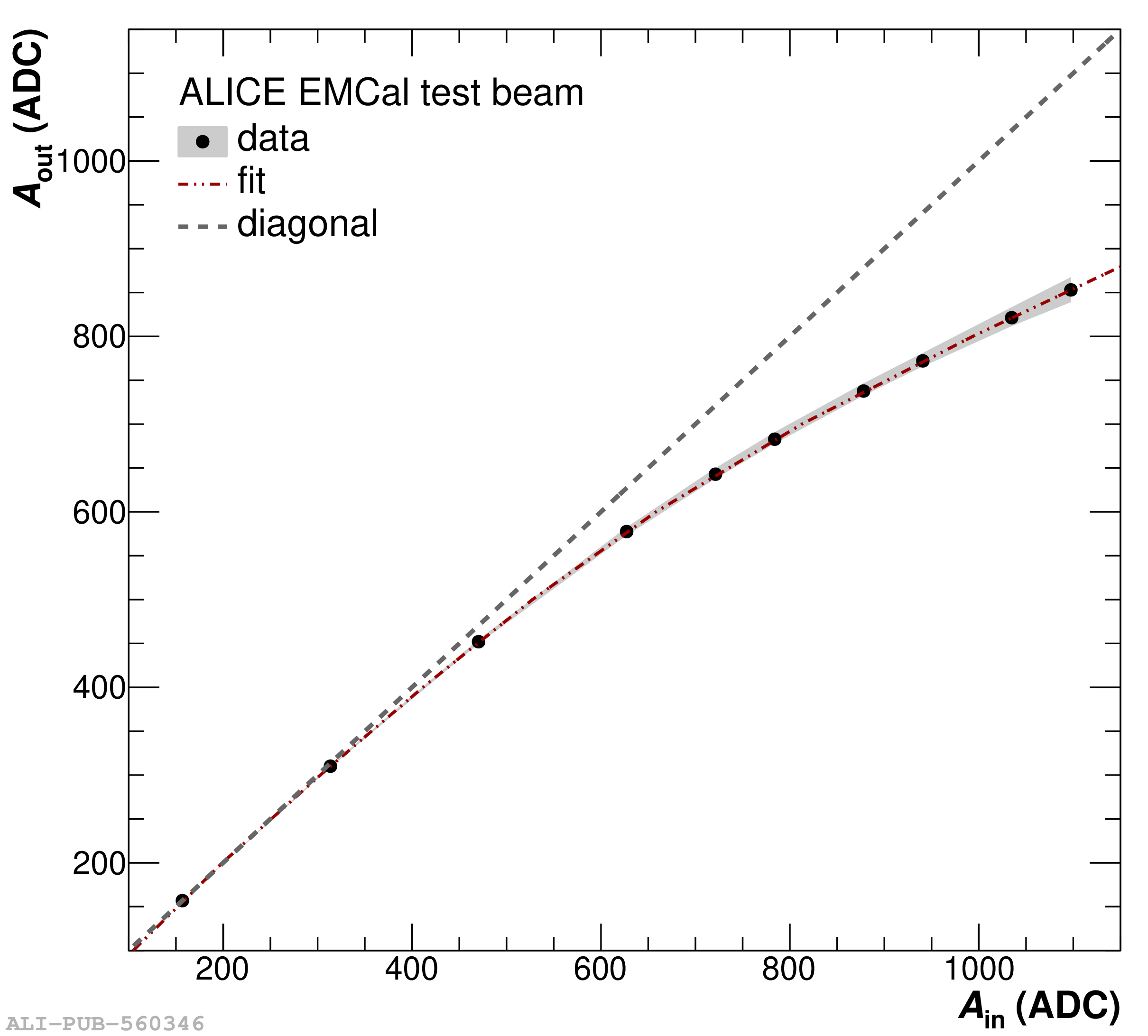 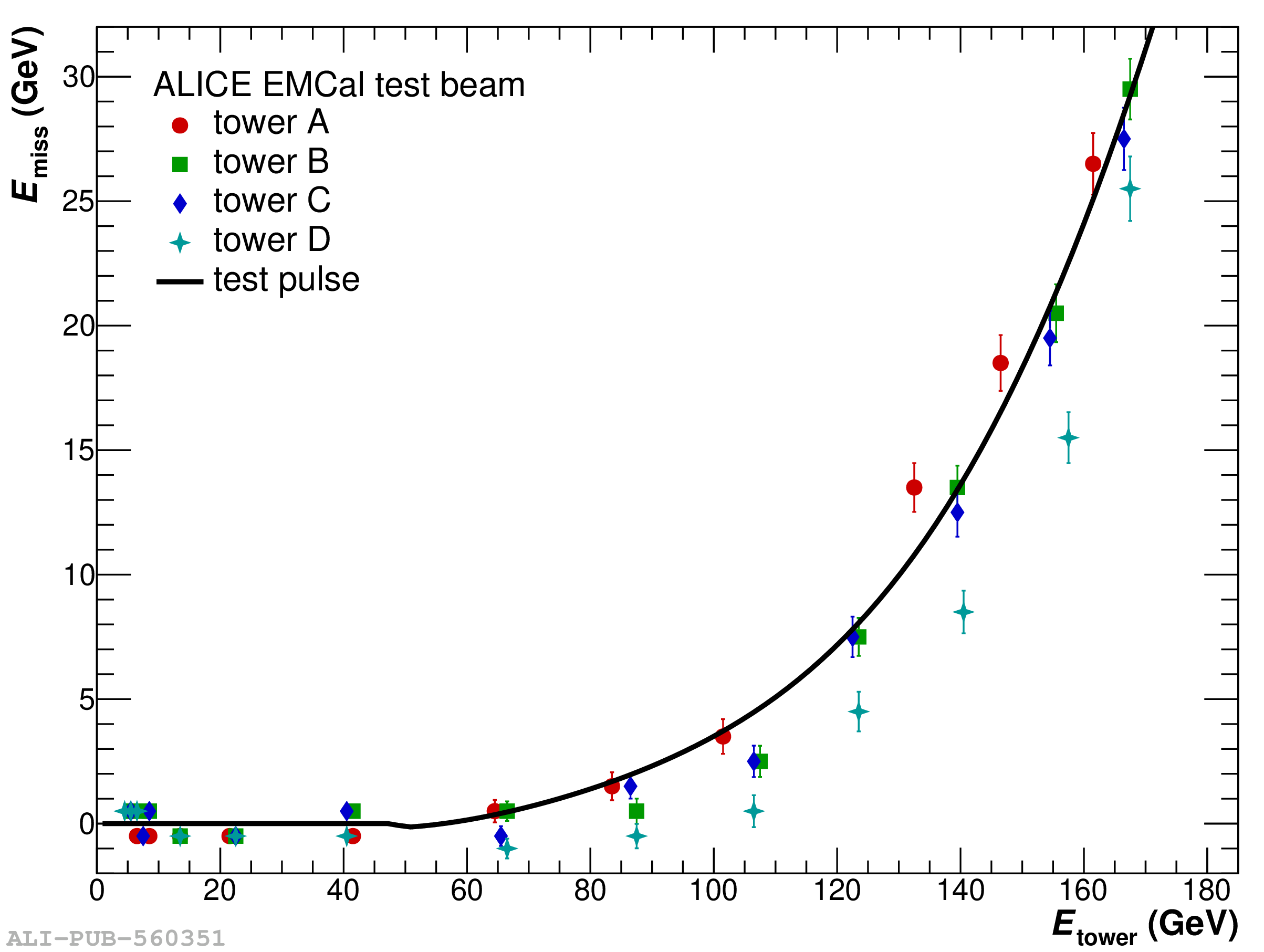 |
Figure 38
Left: energy distribution of single cell clusters obtained from scans with a 6 GeV muon-beam. Right: energy distribution of clusters obtained from scans with a 6 GeV electron beam. For both cases, the data are shown with black markers and compared with the predictions from MC simulations with GEANT3 and GEANT4 transport codes. | 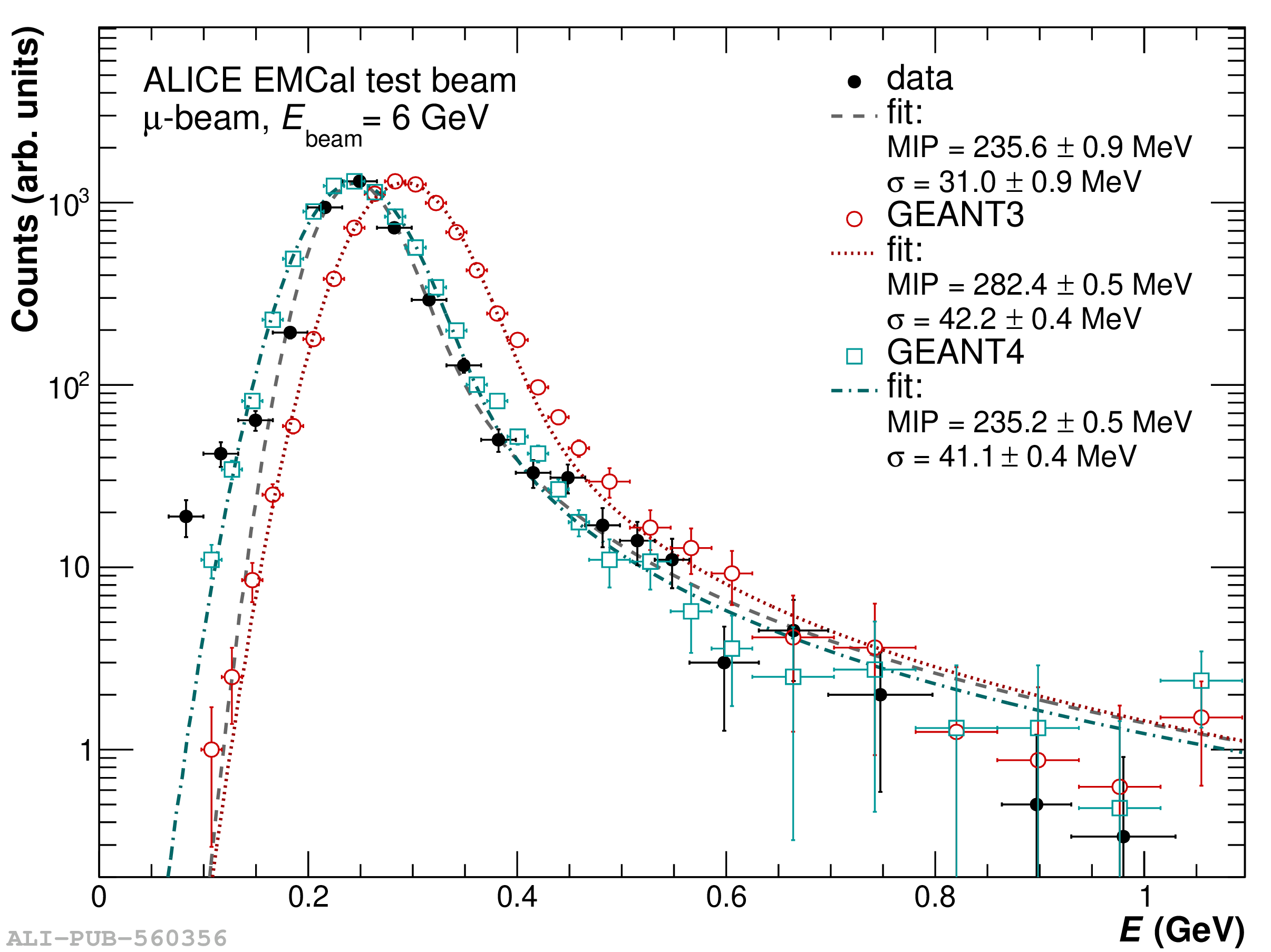 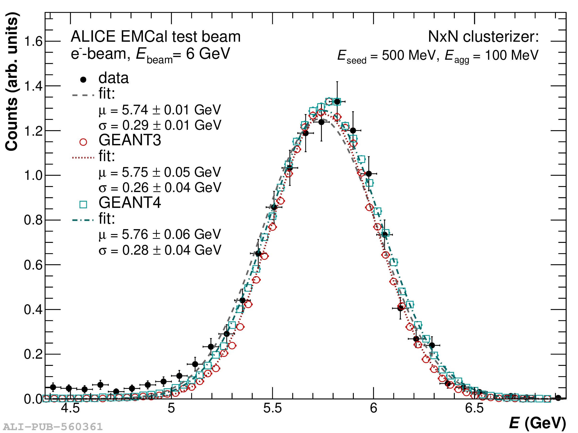 |
Figure 39
Cluster reconstruction/finding efficiency (left) and energy nonlinearity (right) as a function of hit position obtained from MC simulations for 1 GeV electrons. Red markers stand for single cell clusters ($n=1$), blue markers stand for the clusters made of at least two cells ($n>1$), and the black markers stand for the clusters with any number of cells ($n>0$). | 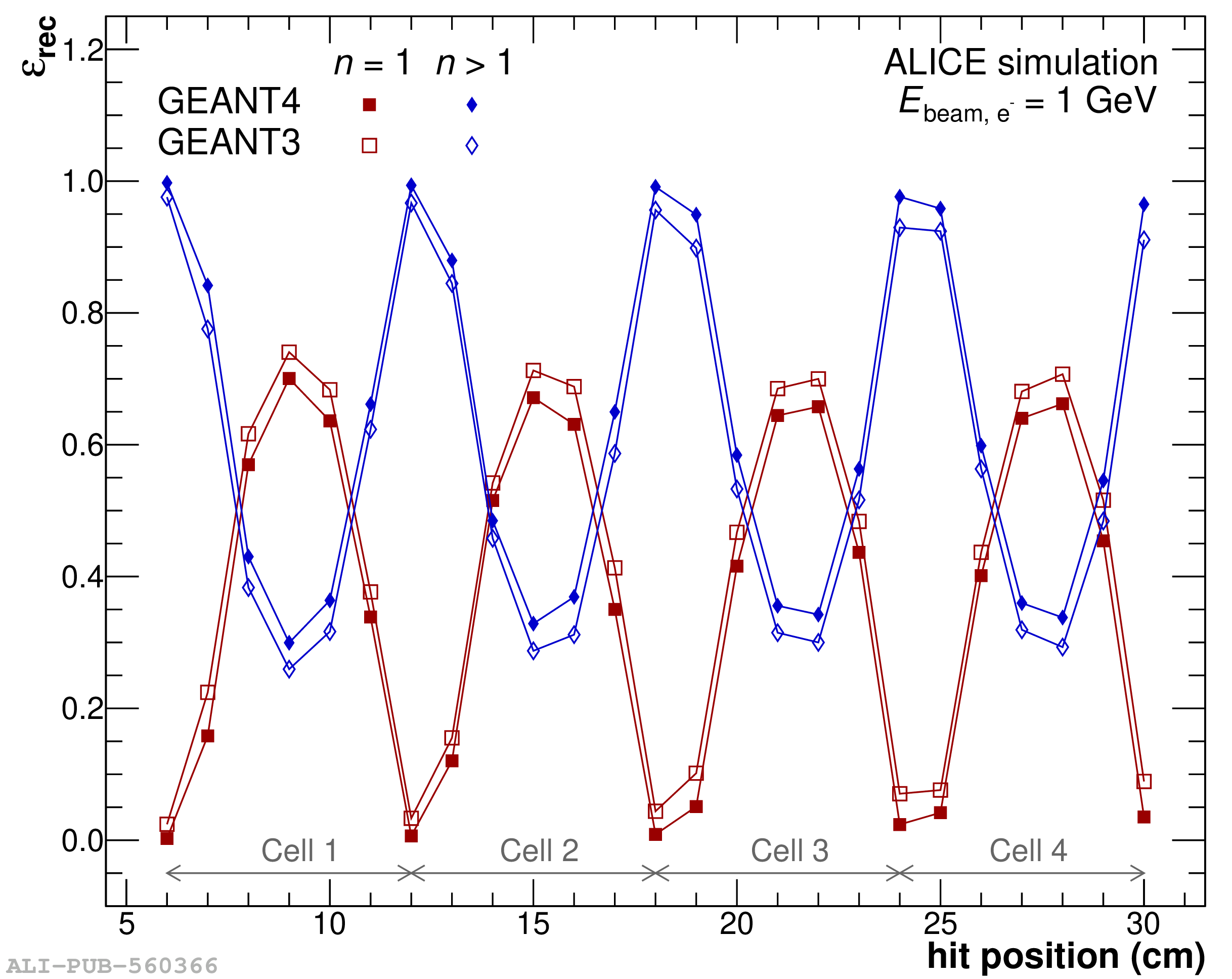  |

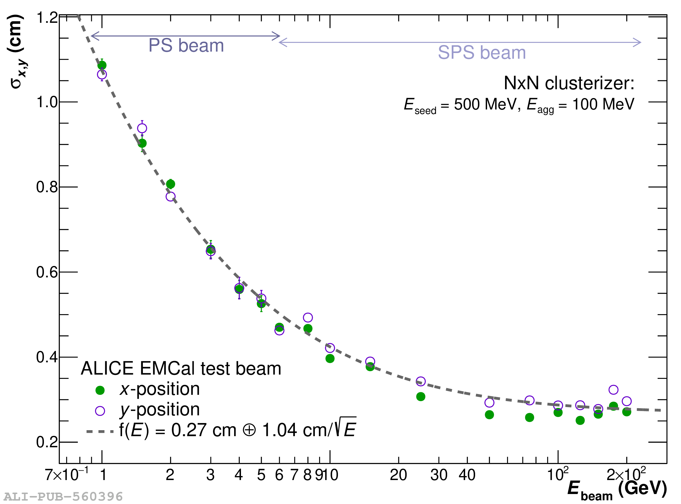
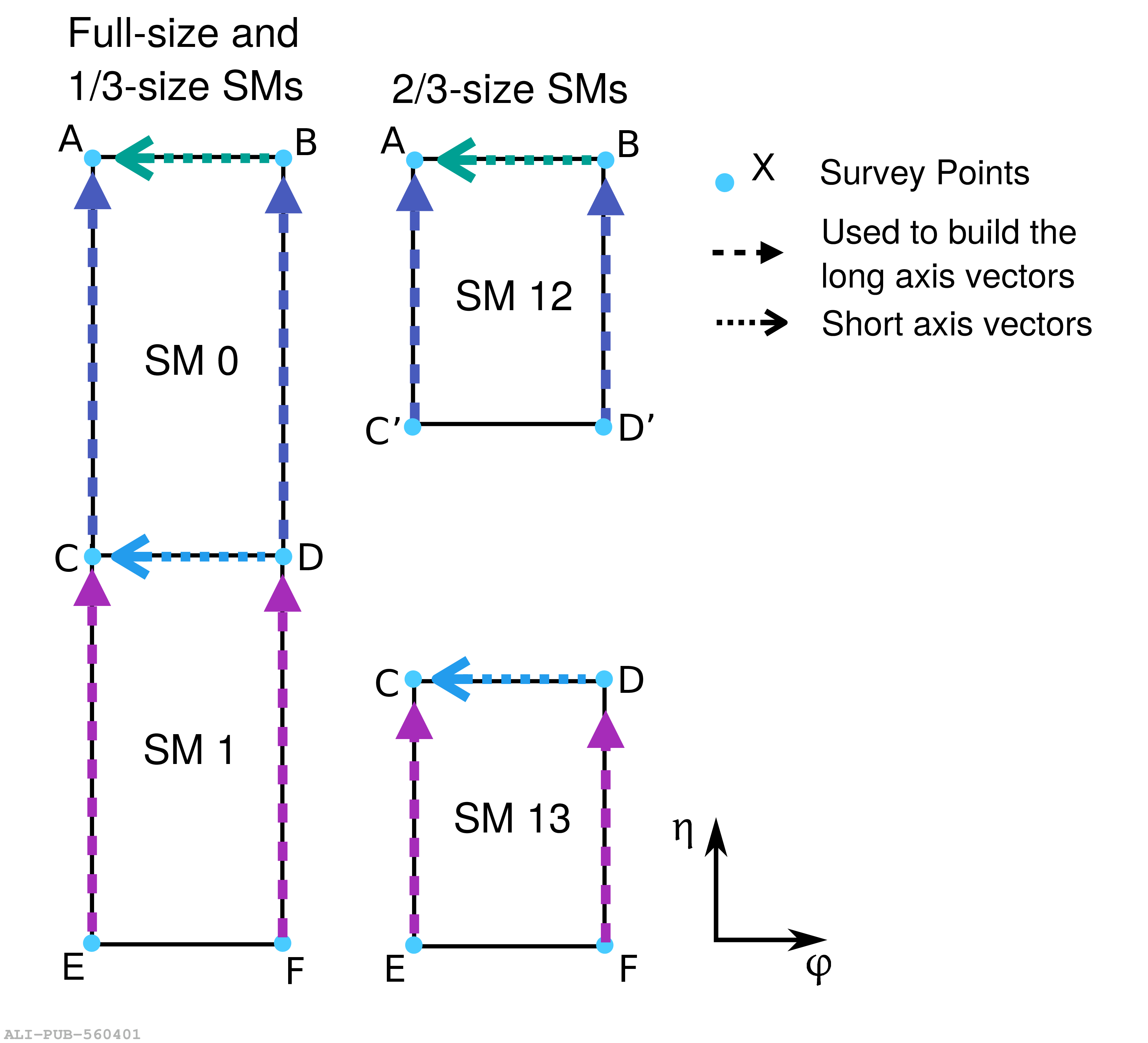


Figure 47
Relative energy resolution as a function of the energy of the incident particle. Displayed are the target resolution (black, dashed-dotted) and the measured energy resolution from the test beam (green, dashed), Sec. 4.3.2. Additionally, three different bands are added showing the intrinsic resolution with added 1, 2 and 3% miscalibration, considering the residual miscalibration during the test beam to be between 0% (upper band limit) and 1% (lower band limit). |  |
Figure 48
Left: Width of the distribution of $\Delta \mu_i$ (see text) as a function of the number of $\pi^{0}$ mesons in sample $S2$, for SMs 0$-$9 (blue, green, cyan) and SMs 10$-$17 (red, orange, yellow), for various $\sigma_{\pi^{0}}$ cell selection: 9.6 $< \sigma_{\pi^{0}} < $ 11.0 MeV/$c^2$ (circles), 9.0 $< \sigma_{\pi^{0}} < $ 12.0 MeV/$c^2$ (diamonds) and none (stars). Right: Statistical uncertainty on the $\pi^{0}$ meson mass as a function of the number of $\pi^{0}$ mesons collected in the cell, for SMs 0$-$9 with the tightest (blue) and without (green) selection on $\sigma_{\pi^{0}}$ as well as for SMs 10$-$17 with the tightest (red) and without (yellow) selection on $\sigma_{\pi^{0}}$. | 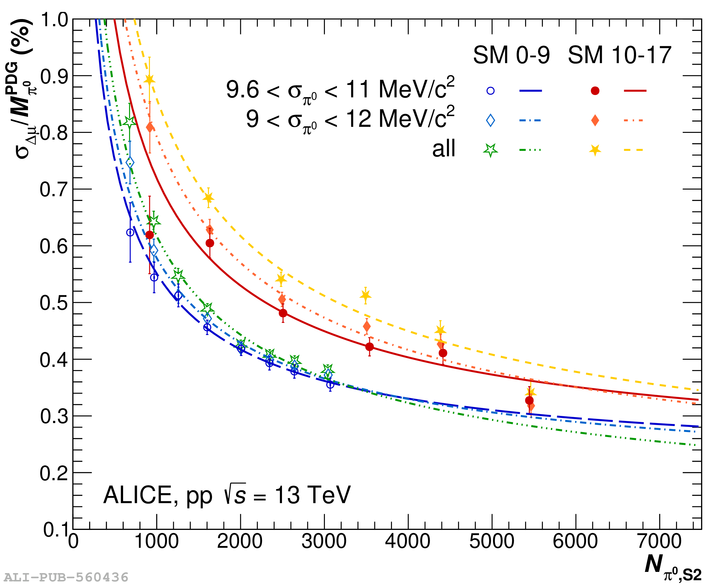 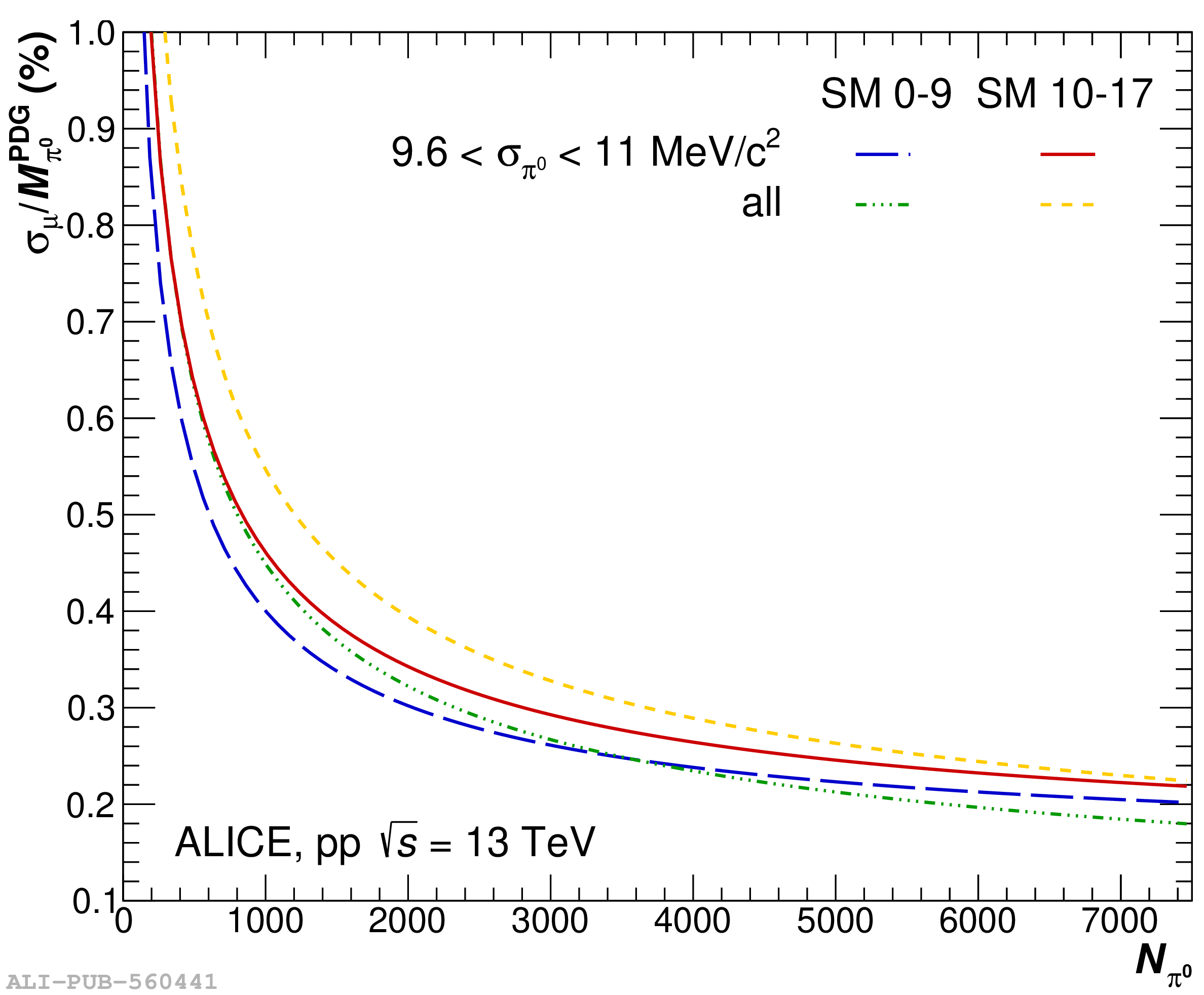 |
Figure 49
Distribution of the ratios of the $\pi^{0}$ meson masses found by a fit in the narrow interval ($\mu^{\text{fit}}_n$) of 70 $< \mu_\pi^{0}< $ 220 MeV/$c^2$ with respect to the standard range ($\mu^{\text{fit}}_s$) of 50 $< \mu_\pi^{0}< $ 300 MeV/$c^2$, for cells located behind the zones with more material (filled distribution) and for the other cells (blue distributions) for SMs 0$-$17. The latter histogram is fit with a Gaussian (red). |  |
Figure 50
Left: Distribution of the number of $\pi^{0}$ mesons collected in an ideal calorimeter (black). The respective contributions of the 10 EMCal, 6 2/3-sized DCal and 4 1/3-sized SMs are displayed in different colors (see Sec. 2.2). Right: Distributions of the smeared $\pi^{0}$ meson masses normalized by $M_{\pi^{0}}^{\rm PDG}$, when only the statistical uncertainty is applied (closed symbols), and when also the uncertainty due to the fit range is applied (opened symbols). |  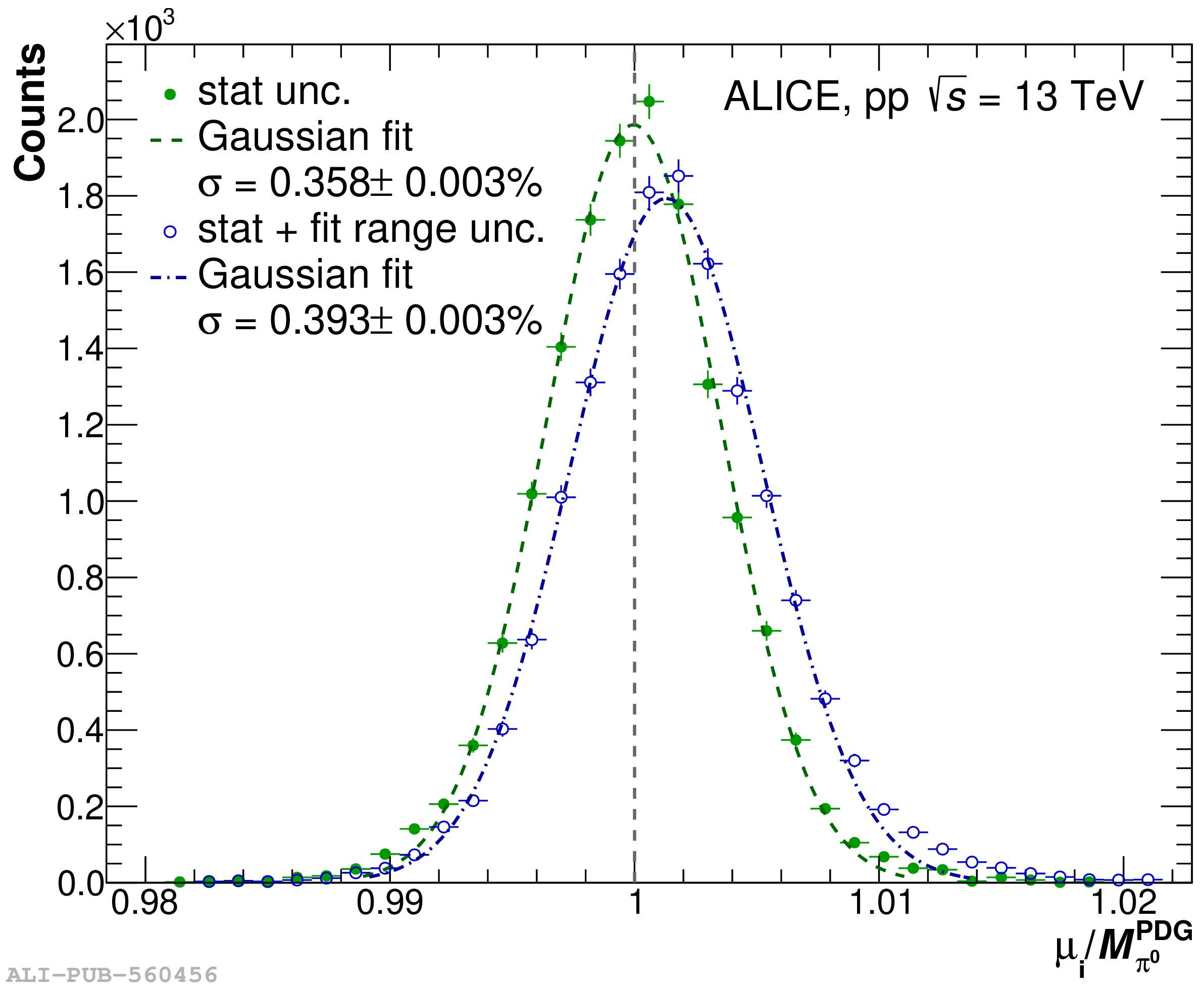 |

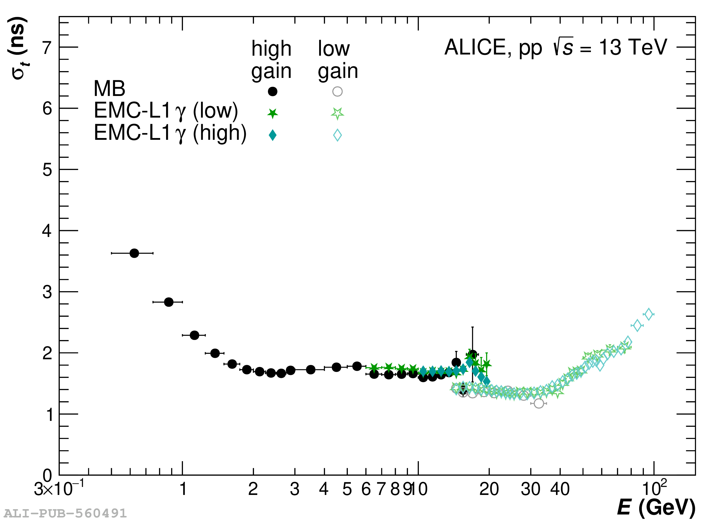
Figure 55
Illustration of the fitting procedure of the normalized LED signal for a good cell in EMCal (left) and a problematic one in DCal (right). The raw distribution obtained for the full 2018 data sample is shown in gray scales in the background, while the maxima in each temperature slice are indicated by green open circles. As there might be multiple clusters of points (as seen on the right) the distribution that is considered as the dominant cluster is marked by black closed circles, while the blue squares represent the shifted distributions after the correction for their offset is applied The final fit to the combined distribution of black and blue points is given as a dashed red line. Points marked in red were iteratively excluded from the fit as they were considered outliers. | 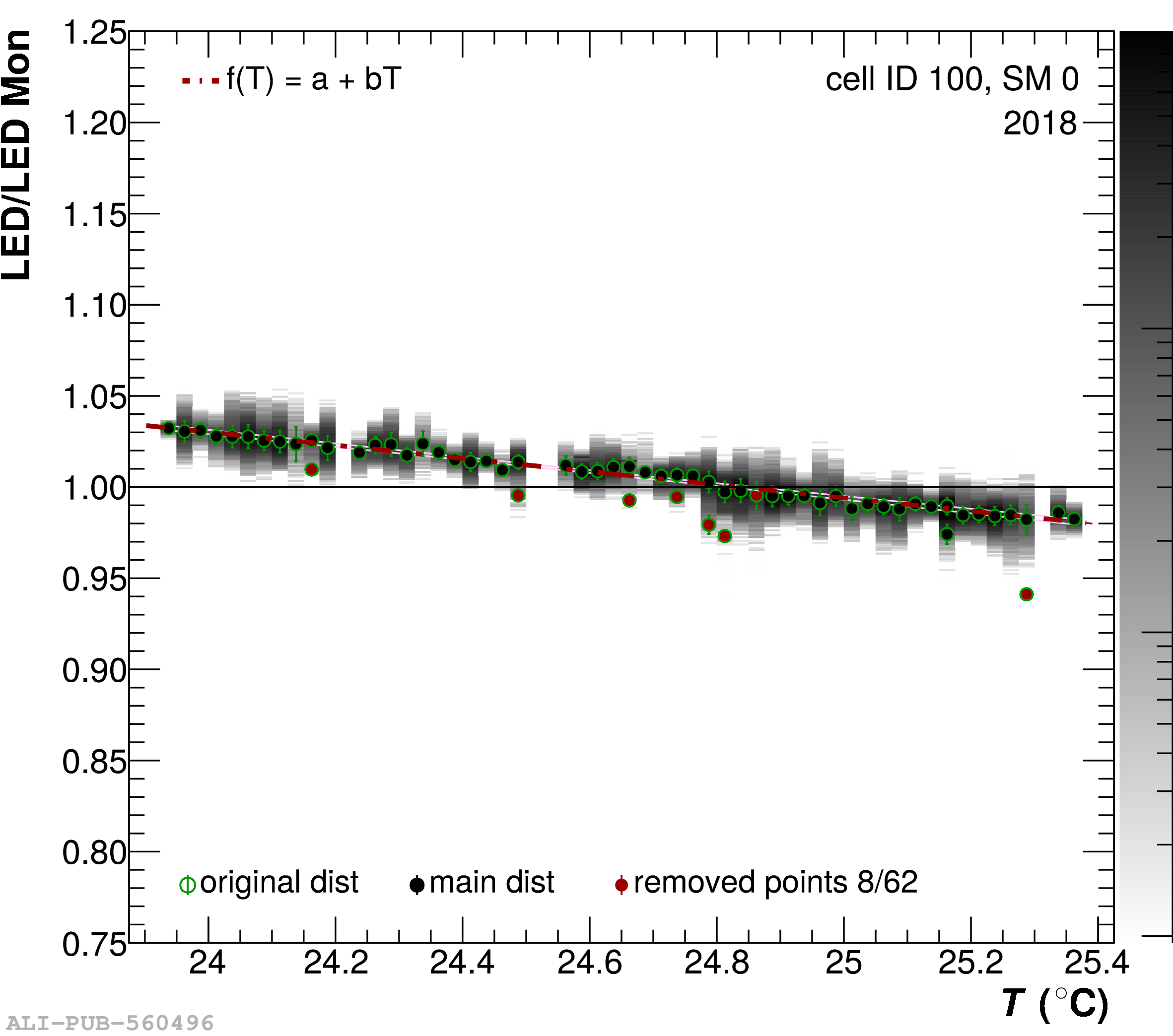 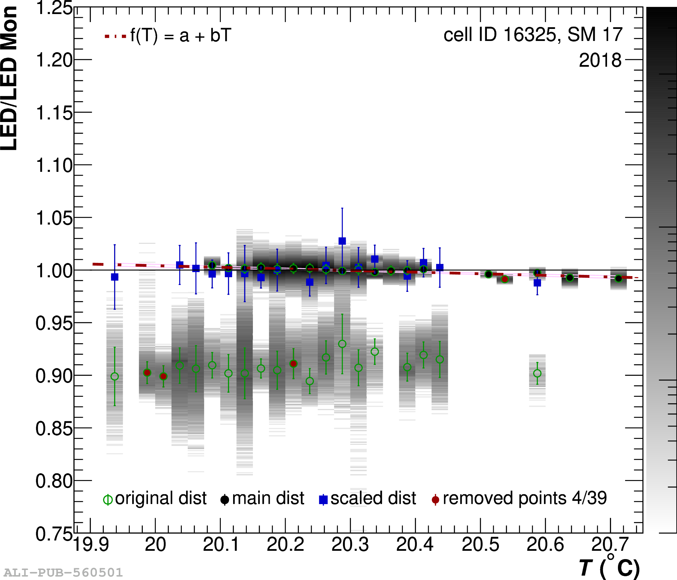 |
Figure 56
Comparison of the obtained temperature calibration parameters in the EMCal (left) and DCal (right). The same cells were chosen as for Fig. 55. The calibration parameters were obtained separately for all years during which the corresponding SM was installed and the cell considered good. The accessible temperature ranges for each year are indicated by the shaded areas in the same colors as the corresponding fits for the respective years. | 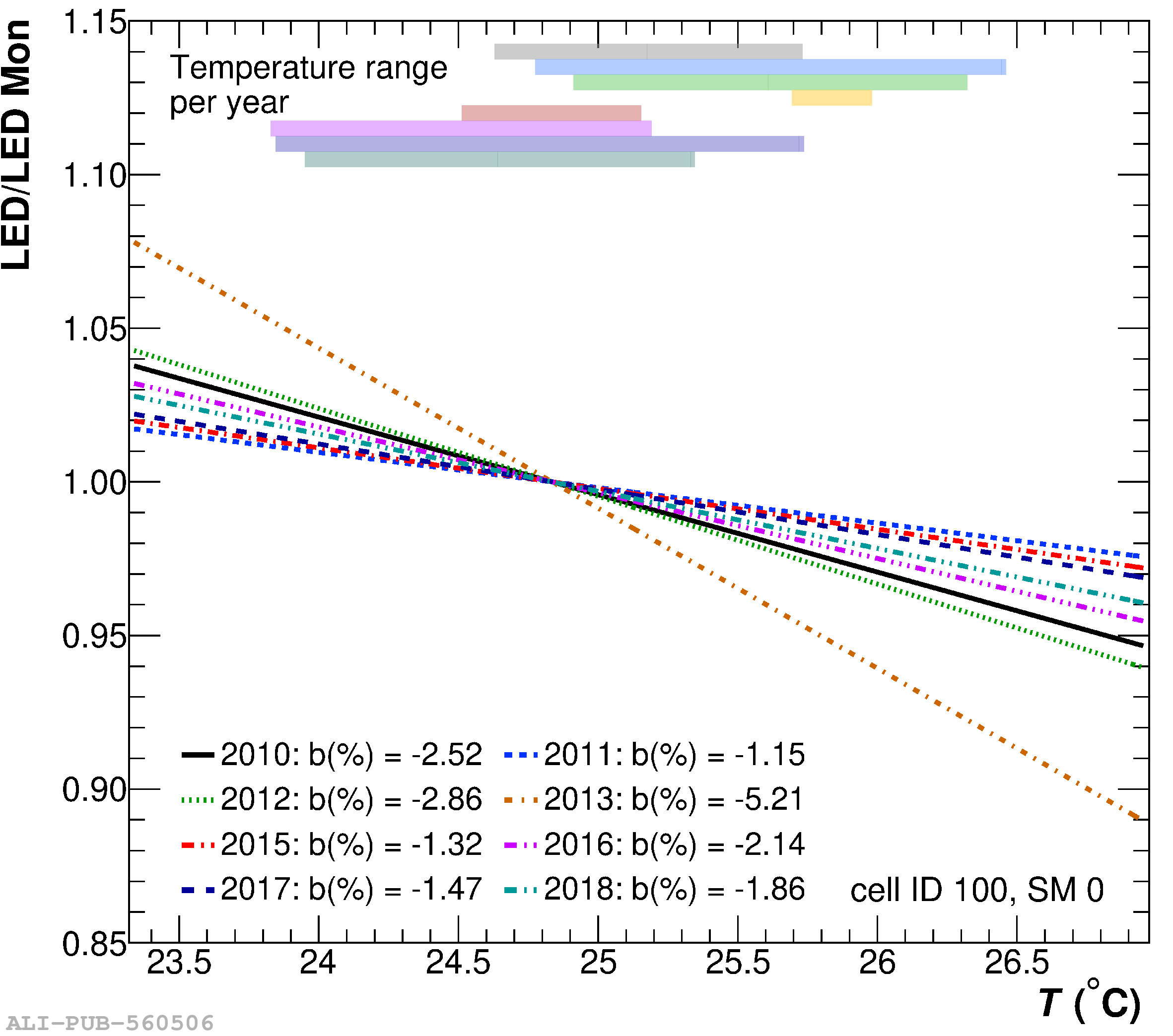 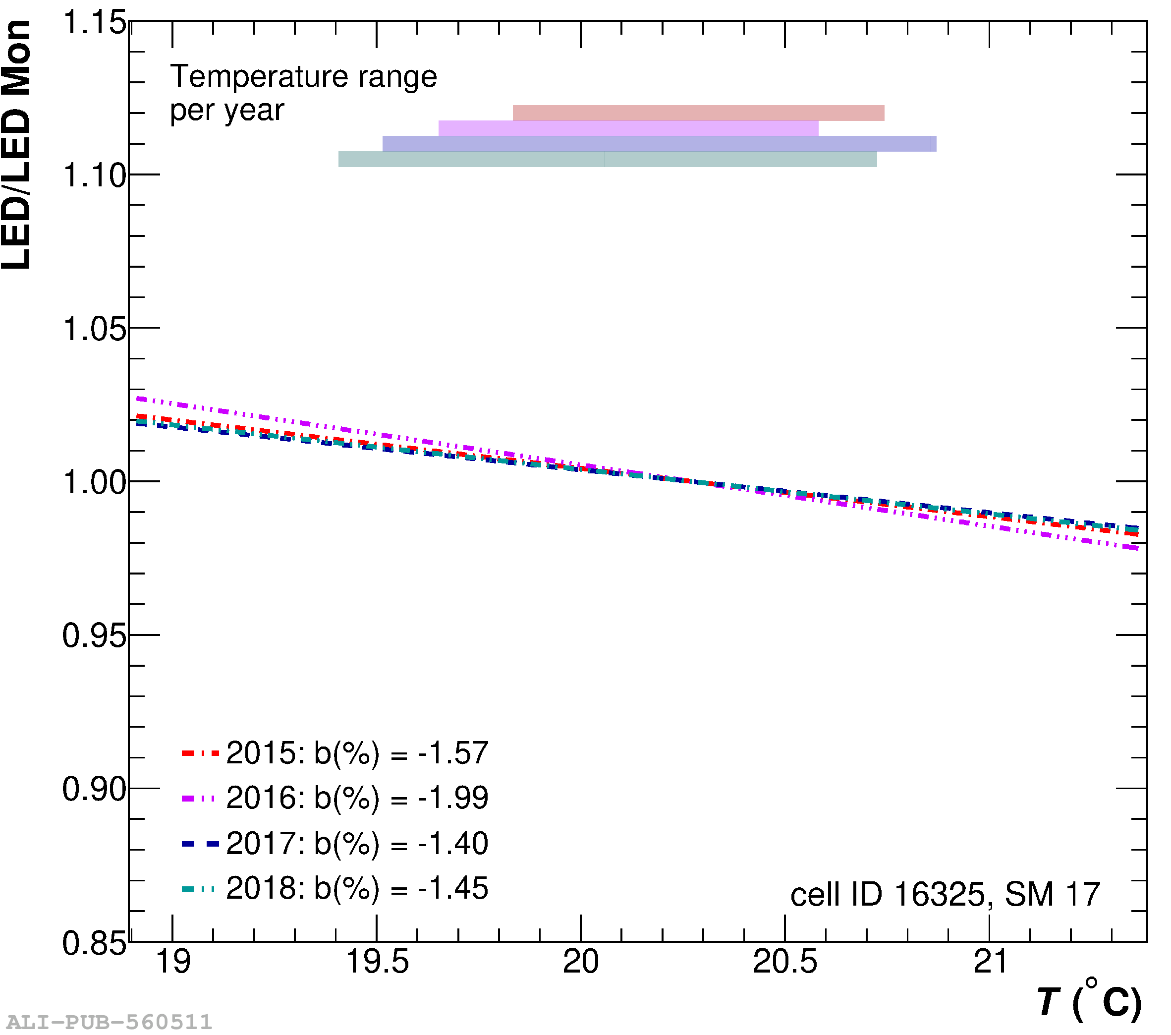 |
Figure 57
Left: Radial distance from the IP of photon conversions in the detector material for different detector configurations in 2010, 2012 and 2015$-$2018. The distributions are obtained for PYTHIA8 simulations and only for photons whose conversion products were reconstructed as clusters in EMCal and formed, when paired with another cluster, a signal in the $\pi^0$ invariant mass window. For 2011 the same number of super modules was installed as in 2012$-$2013, but two fewer modules had the TRD installed in front of them. Right: Neutral pion invariant mass peak position as a function of $p_{\rm T}$ for different magnetic field configurations for pp collisions at $\sqrt{s}=$ 13 TeV. | 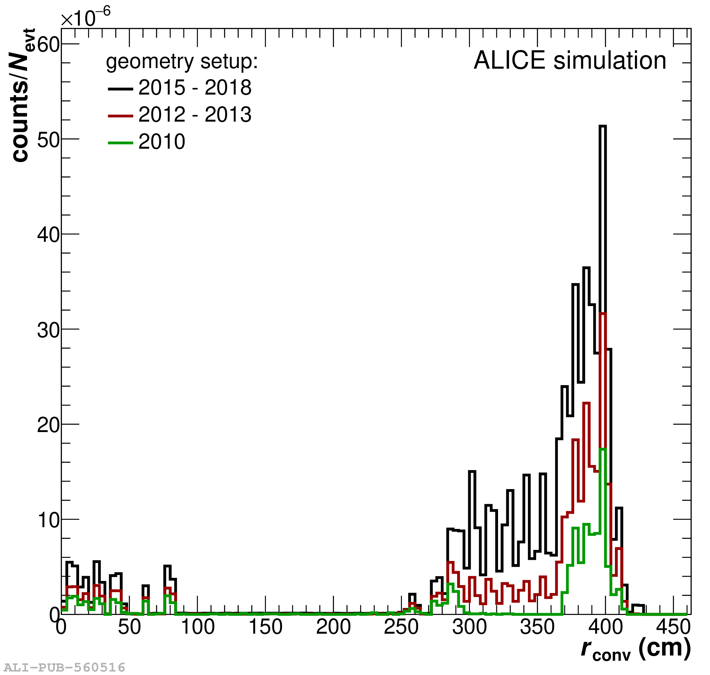 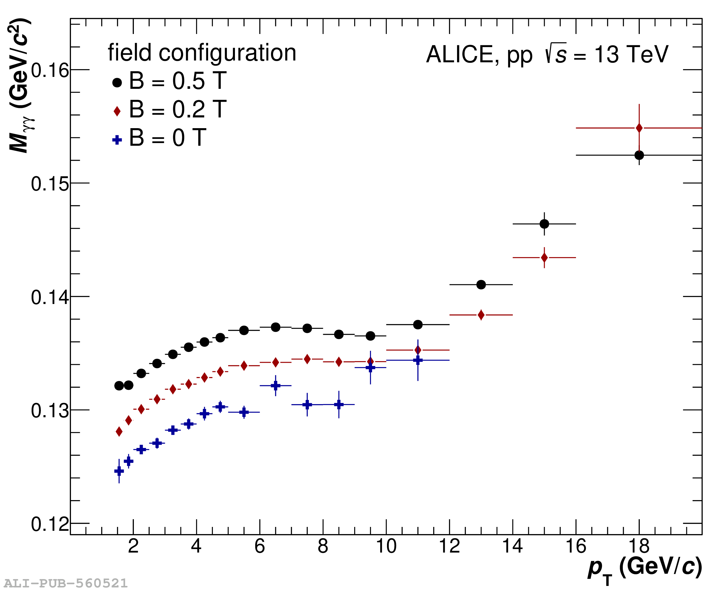 |
Figure 58
Invariant mass distribution of reconstructed $\pi^0$ mesons in MC simulations. Contributions from pure photon pairs as well as from clusters which contain converted photon contributions are shown separately for $B =$ 0.5 T (left), $B =$ 0.2 T (middle) and $B =$ 0 T (right) for pp collisions at $\sqrt{s}=13$ TeV. | 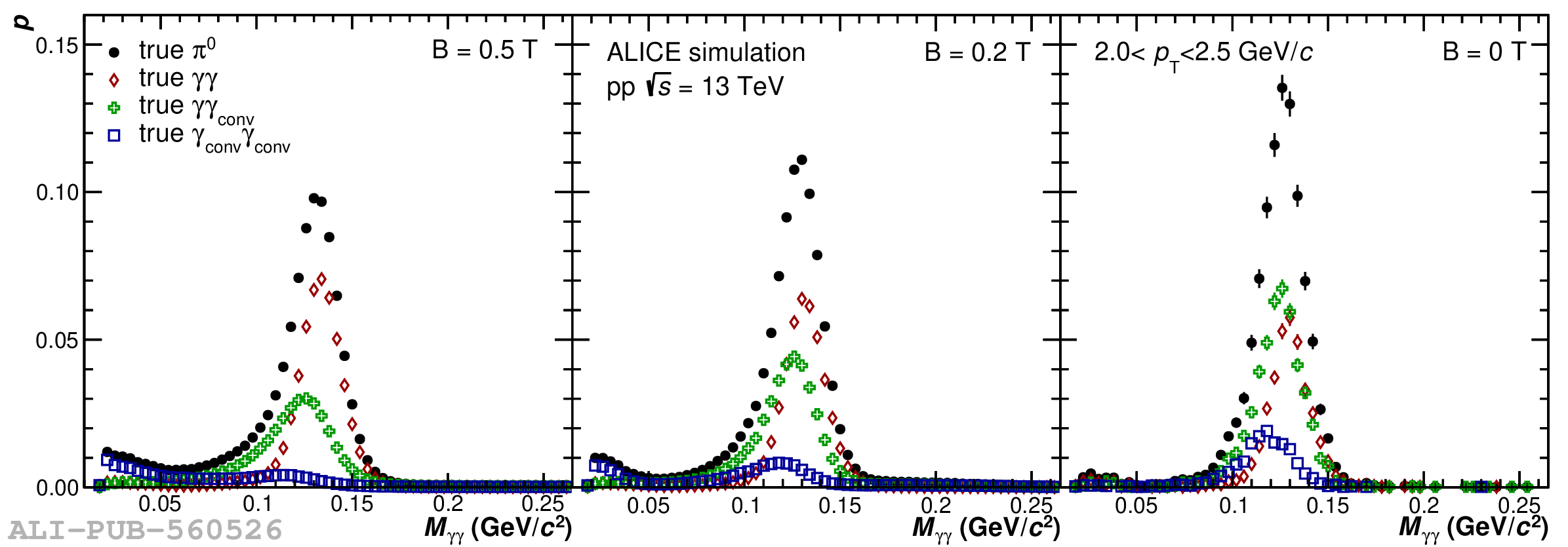 |
Figure 59
Left: Mass positions for PCM-EMC (blue) and EMC (green) after applying the nonlinearity correction obtained from Sec. 4.3.2 Fig. 41. The mass positions are normalized to the neutral pion rest mass. In the case of PCM-EMC the data points represent the squared mass position. Right: Ratio of mass positions in data and MC for both techniques with their corresponding fits according to Eq. 27. | 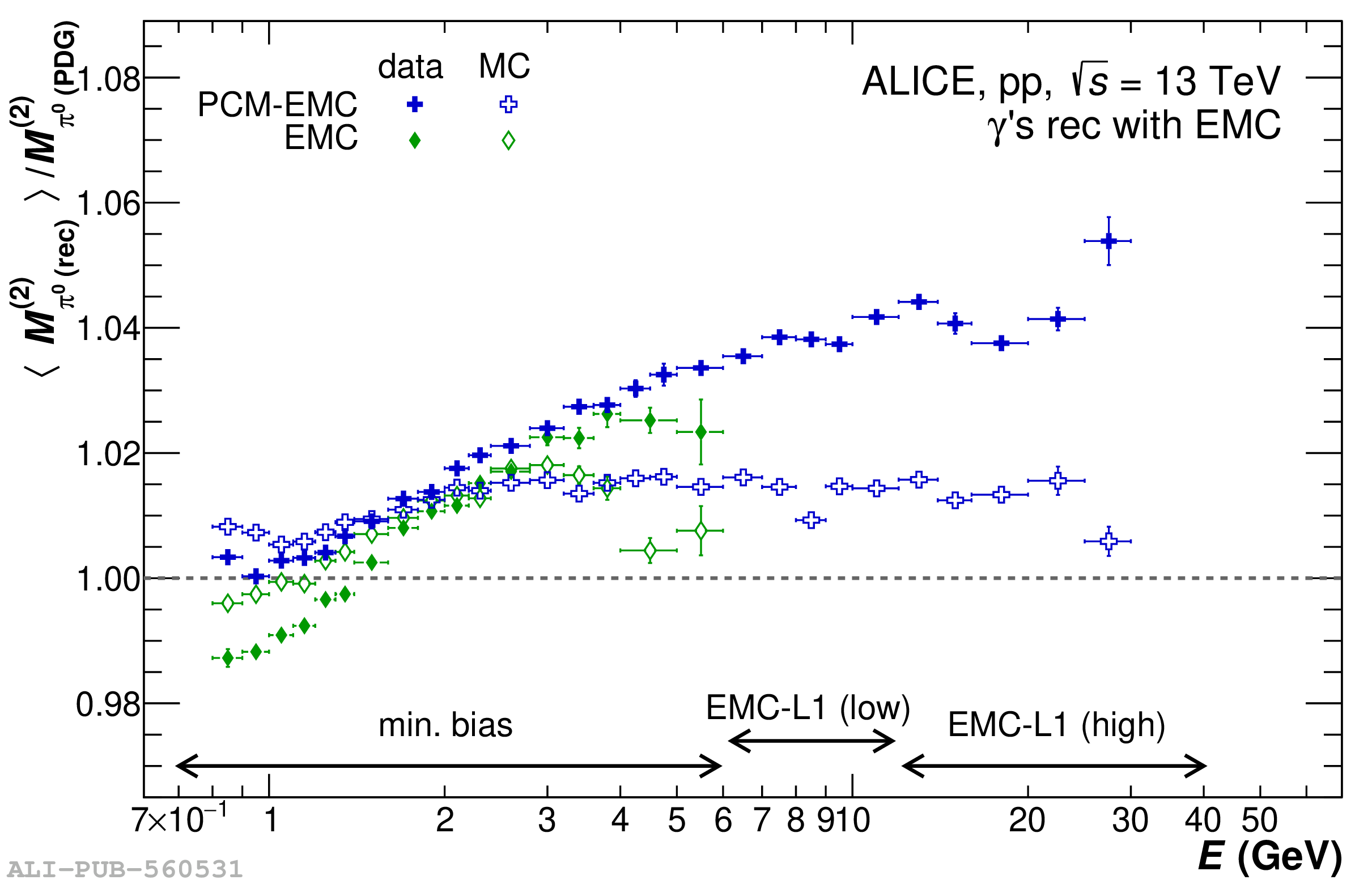  |

Figure 62
Left: Fraction of clusters with 2 or more cells for data and MC for clusters selected with PCM-EMC tagging and EMC tagging. Right: Ratio of fully corrected $\pi^{0}$ meson spectra obtained with PCM-EMC (top) and EMC (bottom) with $N_{\rm{cell}} \geq 2$ to the $N_{\rm{cell}} \geq 1$ with and without applying the cluster-size correction. | 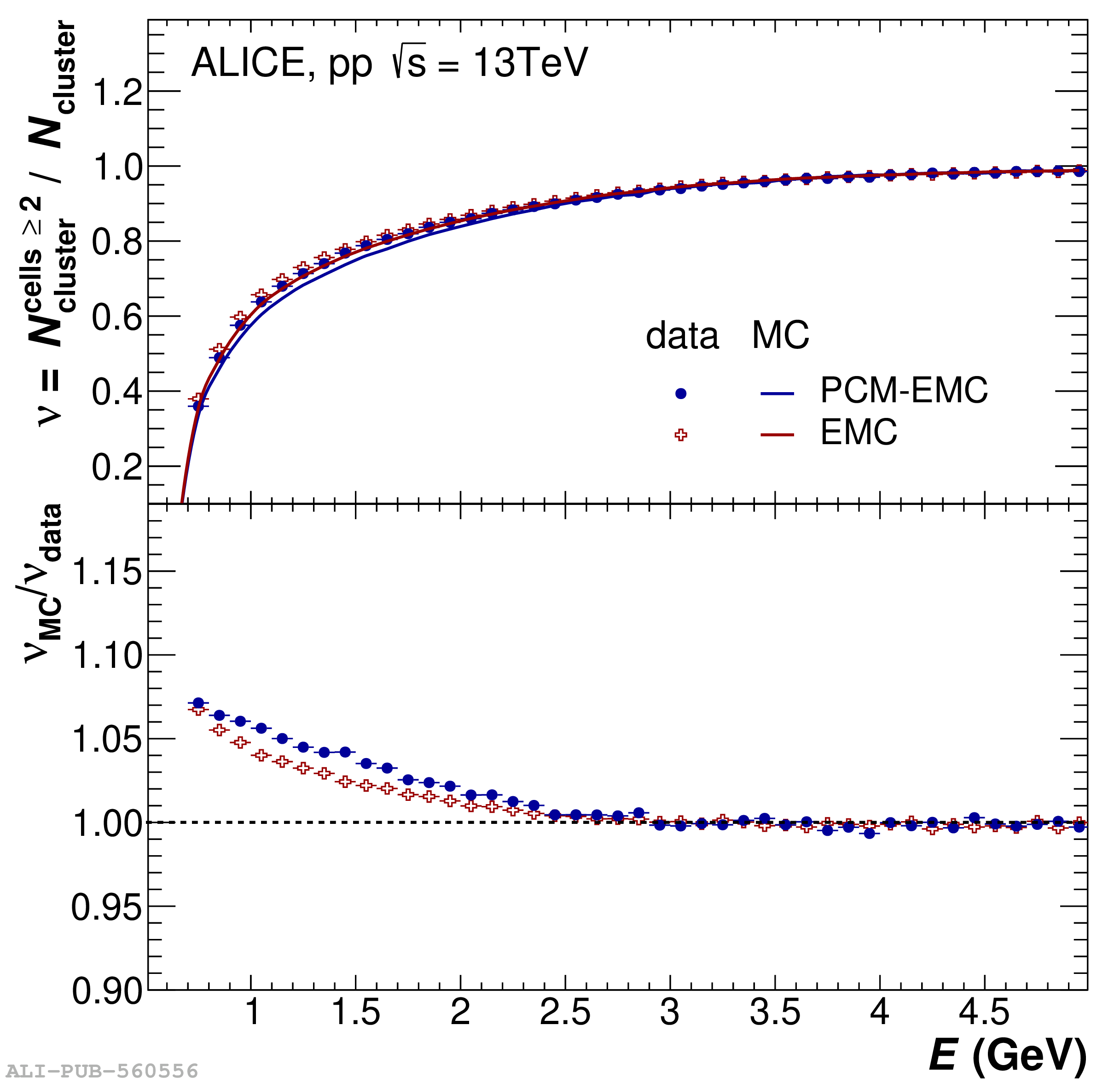 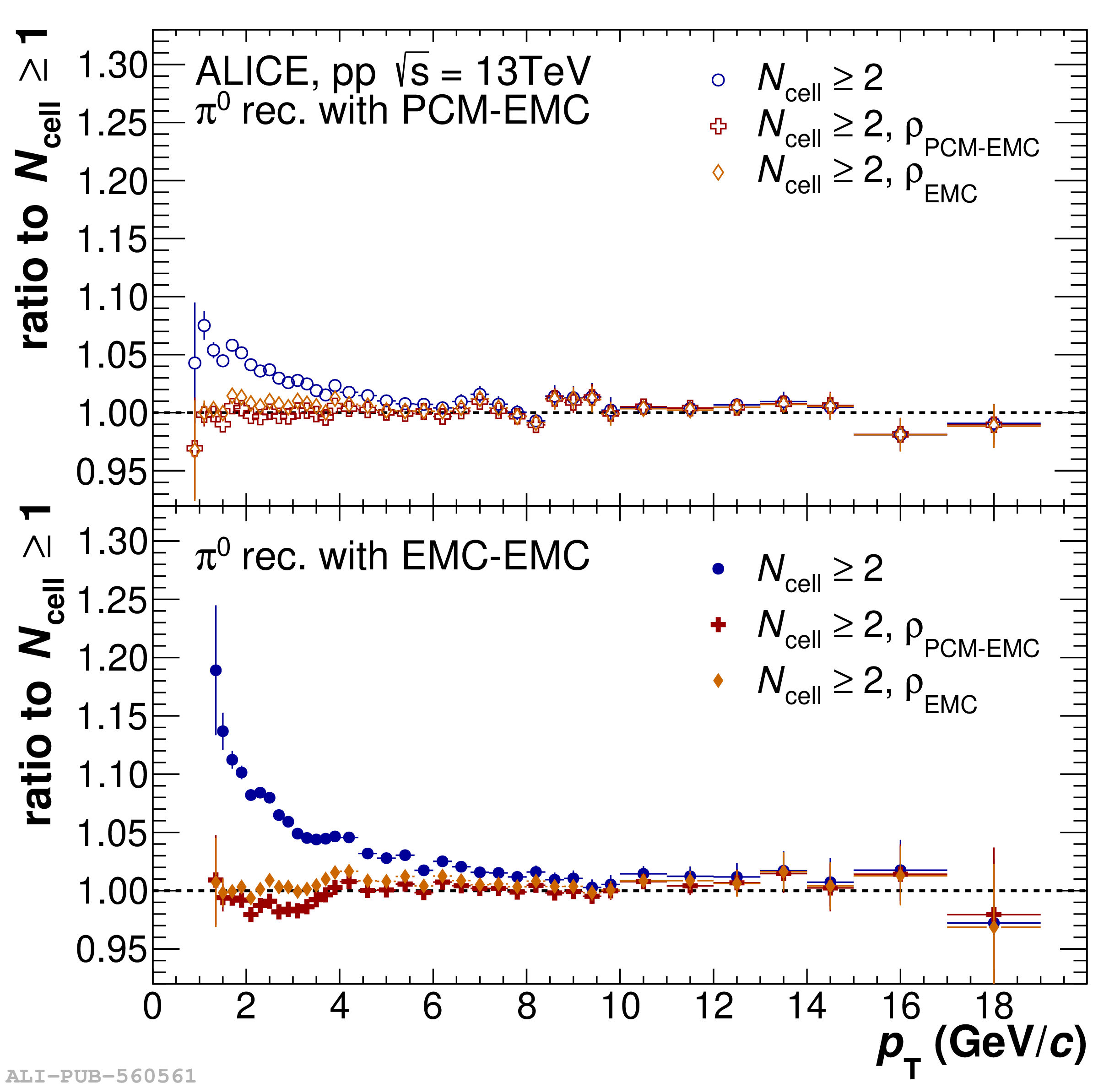 |
Figure 64
Probability distributions of the shower shape parameter $\sigma_{\rm long}^{2}$ of neutral clusters in data and simulations. The different panels show different neutral cluster energy intervals. All distributions are normalized to their integral. Data are shown as black histograms and simulations PYTHIA6 events with two jets or a direct photon and a jet in the final state, with GEANT3 default settings) in blue. For the red histograms the modelling of the cross-talk observed in the EMCal electronics was included in the simulations. | 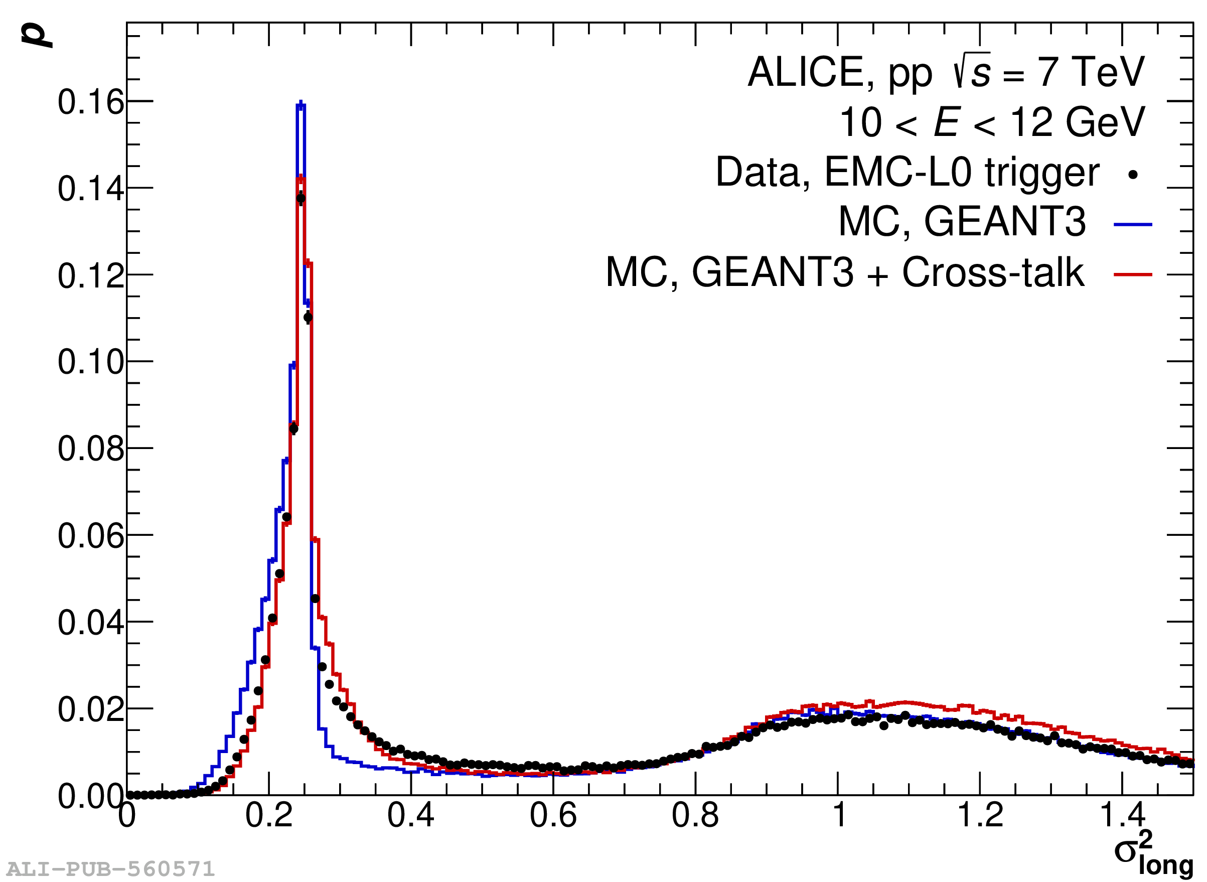 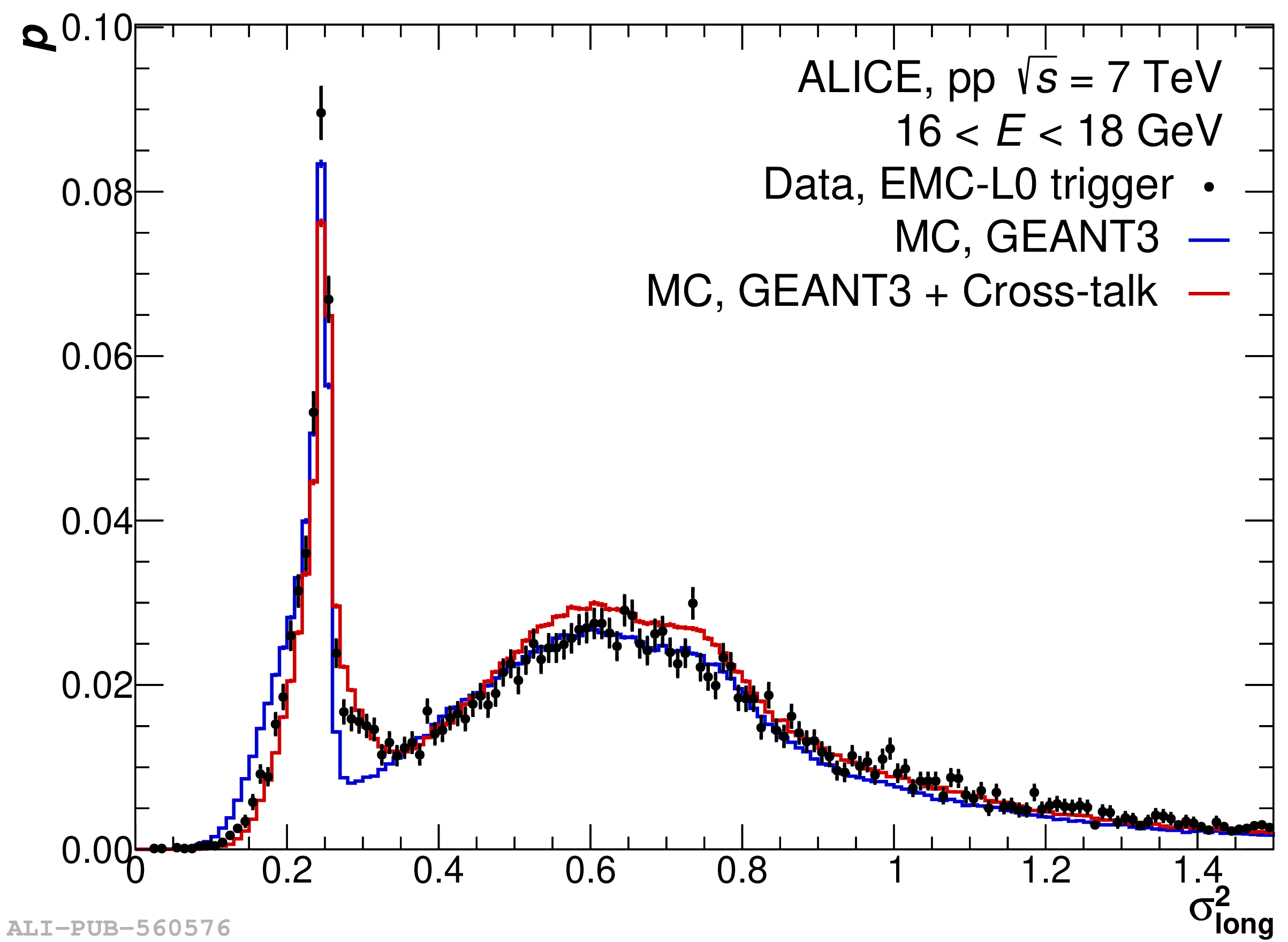  |
Figure 65
Comparison of the probability distribution of the shower shape parameter, $\sigma_{\rm long}^{2}$, of neutral clusters with $n^{\rm w}_{\rm cell}>1$ (left) and $>4$ (right) for different fractions of induced energy in the cross talk model (see Eq. 29), in pp collisions at $\sqrt{s}=$ 7 TeV EMCal triggered data are compared to PYTHIA6 simulated events with a direct photon and a jet or two jets in the final state, where one jet is triggered by a decay $\gamma$ on EMCal acceptance with $p_{\rm T}>$ 3.5 GeV/$c$. Data and default MC (untuned simulation) are the same as in Fig. 64. |  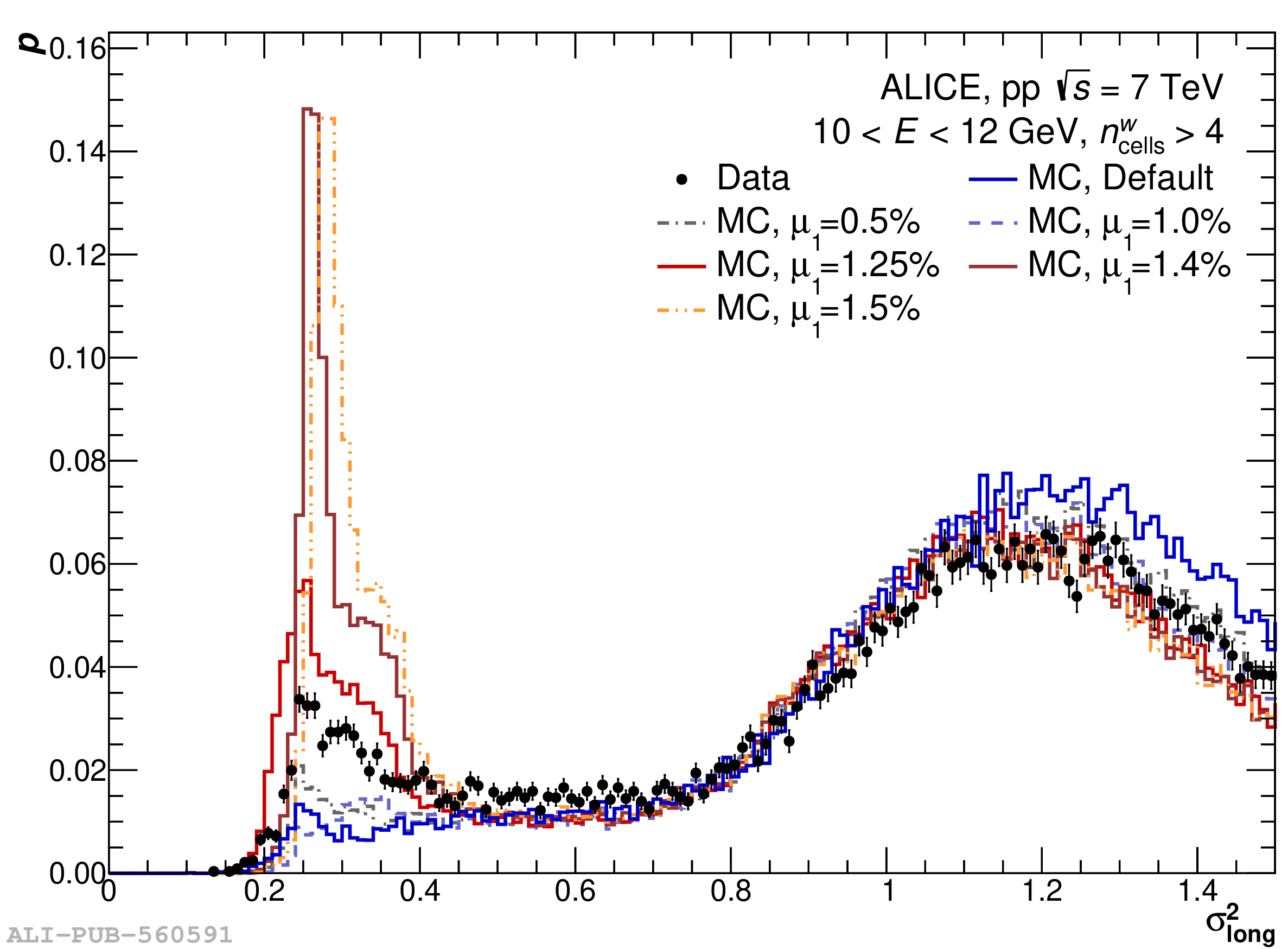 |
Figure 66
Fraction of clusters with $n^{\rm w}_{\rm cell}>4$ within the range $0.1< \sigma_{\rm long}^{2}< 0.3$ per SM. Left and middle: pp $\sqrt{s}=$ 13 TeV L1 $\gamma$ triggered data. Right: Clusters (enhanced merged decay population by few %) in EMCal for pp $\sqrt{s}=$ 7 TeV minimum bias and L0 trigger data (black marker), compared to simulations with 2 jets in the final state with different photon trigger thresholds, with (red marker) and without (blue marker) cross-talk tuning. |  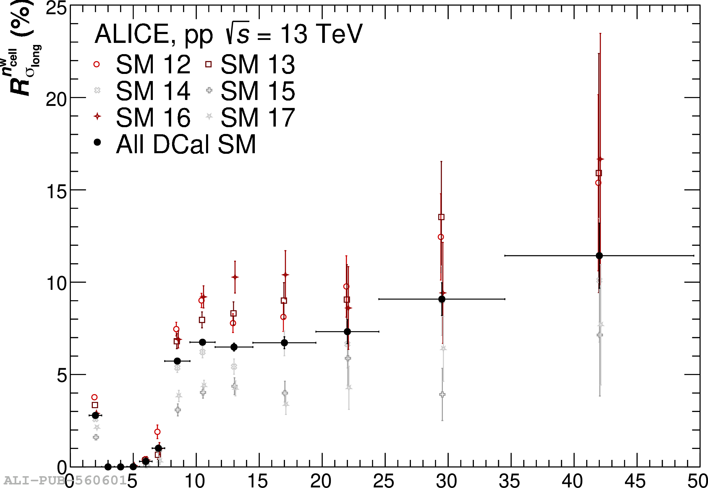 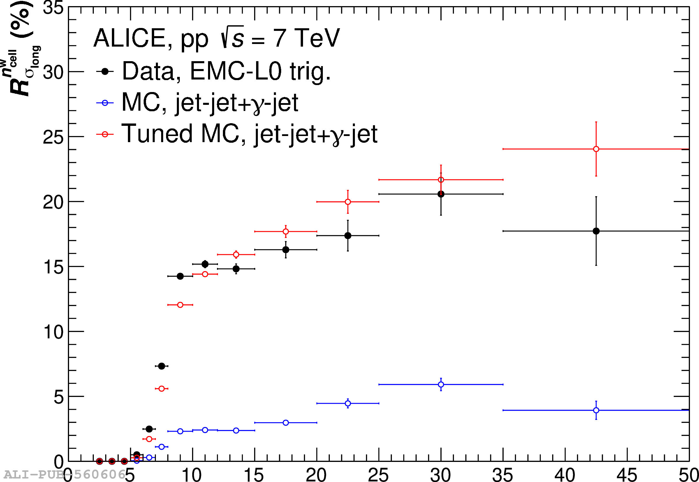 |
Figure 67
Left: $\sigma_{\rm long}^{2}$ as a function of the cluster energy. Data, pp collisions at $\sqrt{s}=$ 13 TeV triggered by the EMCal and DCal with L1-$\gamma$ at $8.5$ GeV, V2 clusterizer. Right: Number of cells in the cluster in the same T-Card as the highest energy cell as a function of the number of cells in a different T-Card, for clusters between 100 and 200 GeV. |  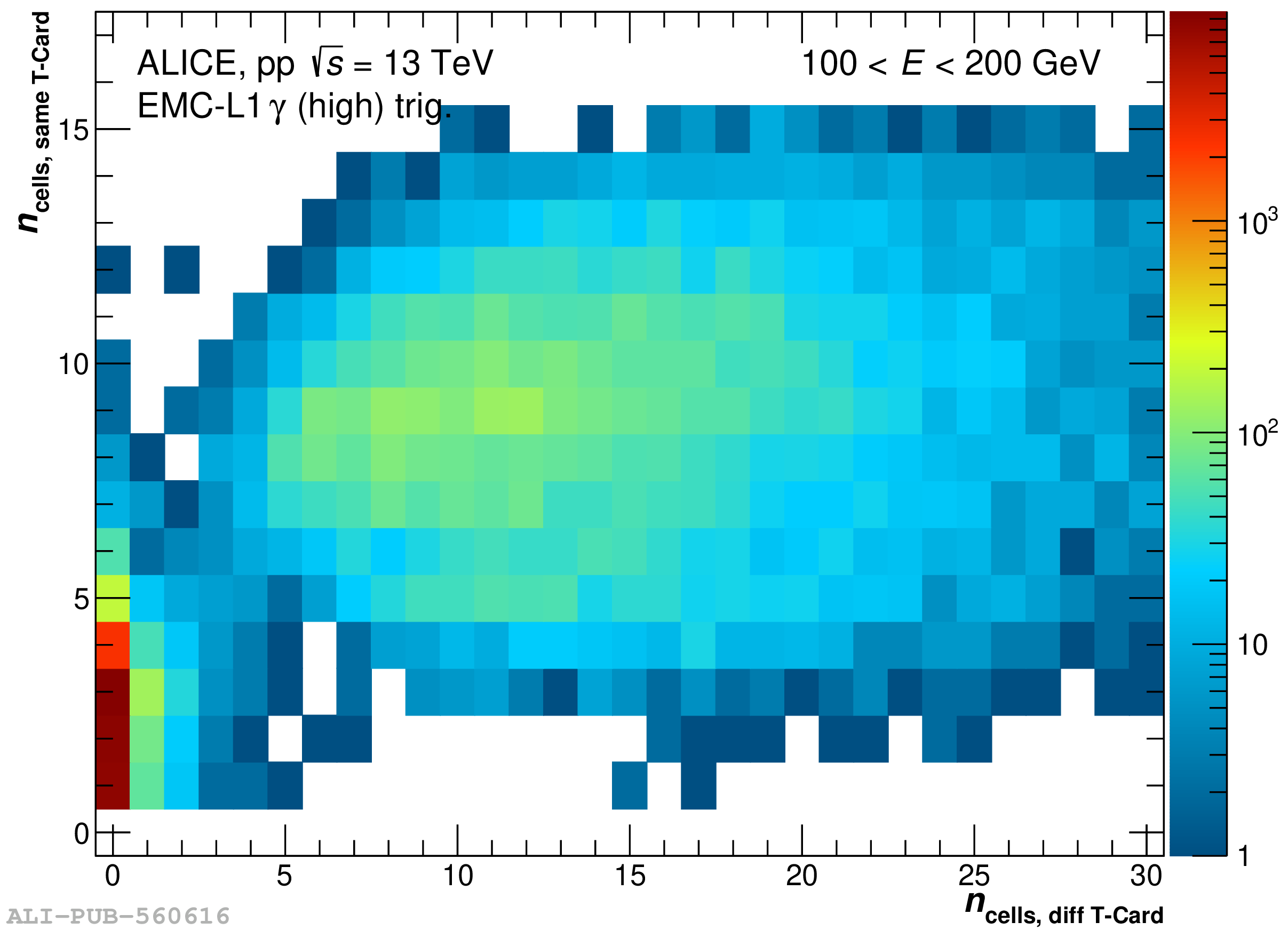 |
Figure 68
Comparison of the probability distributions between data and simulation for cluster $n_{\rm cells}$ (left), $F_{+}$ (middle) and $\sigma_{\rm long}^{2}$ (right) for V2 clusters with $75 < E < 100$ GeV. Selections applied: reject clusters with no cell in a different T-Card as the highest energy cell, $F_{+}>0.95$ and $\sigma_{\rm long}^{2}>0.1$ where it applies. Data and simulation of pp collisions at $\sqrt{s}=$ 13 TeV, simulation of PYTHIA8 events with two jets or a direct photon and a jet in the final state, and with cross talk emulation activated (red points) and not activated (blue points). |    |
Figure 69
Left: Ratio of the number of selected clusters after each applied selection with respect to basic cluster selections (see Tab. 6) as a function of the cluster momentum. The green markers indicate the use of the CPV requirement, while the red markers include the CPV and $\sigma_{\rm long}^{2}$ selection criteria. For each step, the data are represented by the points, while the lines indicate the same selection step in the simulations. Right: Inclusive photon purity $P$ and reconstruction efficiency $\varepsilon_{\gamma}$ as defined in Eqs. 30 and 31 after applying each cluster selection criterion. Both figures are done using V2 clusters as inputs. | 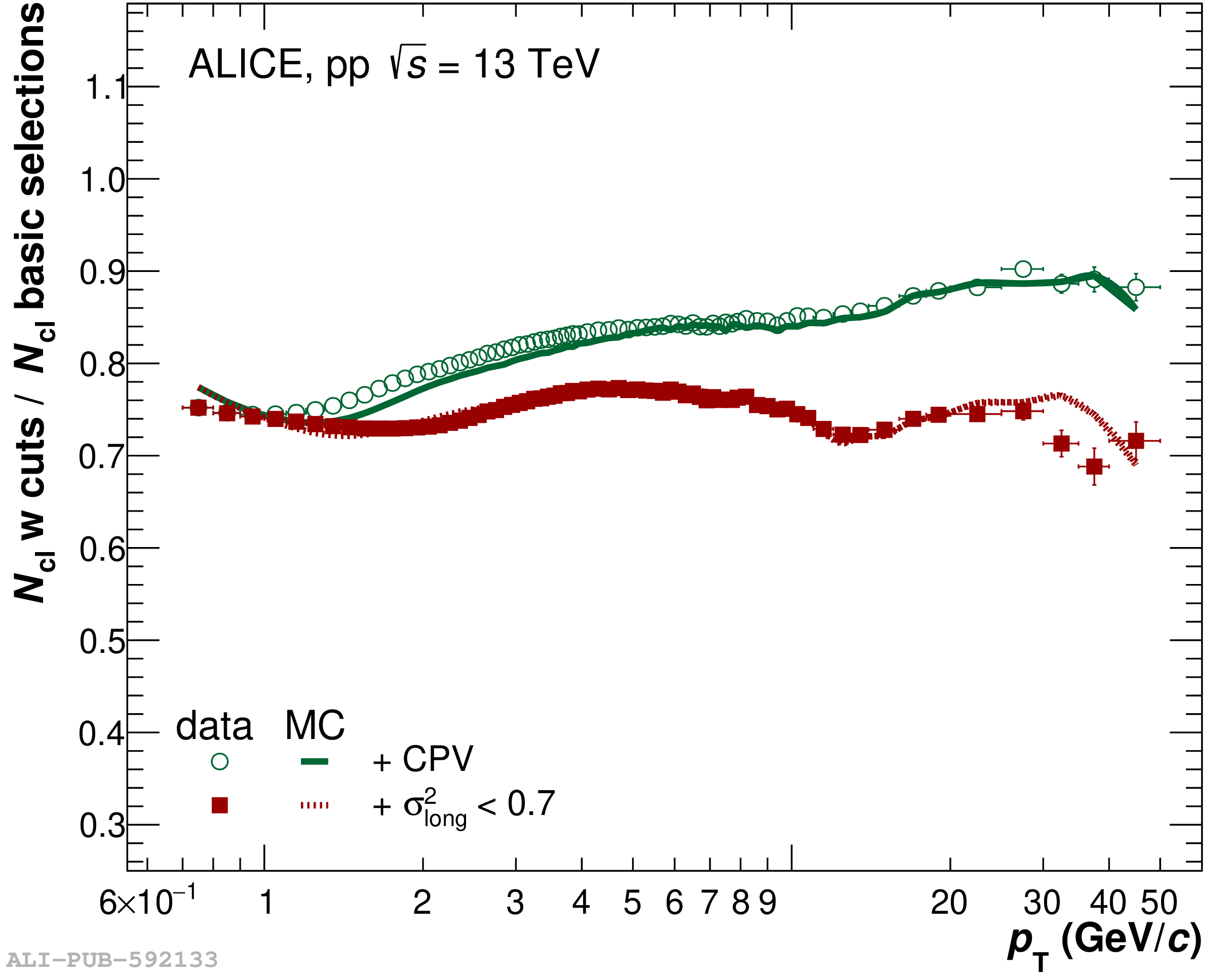  |
Figure 70
Comparison of the purity (left) and reconstruction efficiency (right) for inclusive photons for the V1 (lines) and V2 (points) clusterizers. The two quantities are shown for a tight (0.1 $< \sigma_{\rm long}^{2}< $ 0.3, red) and loose (0.1 $< \sigma_{\rm long}^{2}< $ 0.7, blue) shower shape selection. |   |

Figure 72
Left: Comparison of the transverse momentum smearing correction ($C_{\rm res}$) contained in the photon efficiency for the V1 (lines) and V2 (points) clusterizers in pp collisions at $\sqrt{s} = 13$ TeV. The different colors indicate different shower shape selections Right: Relation between reconstructed cluster and true photon momenta for photon candidates reconstructed with the V2 clusterizer. | 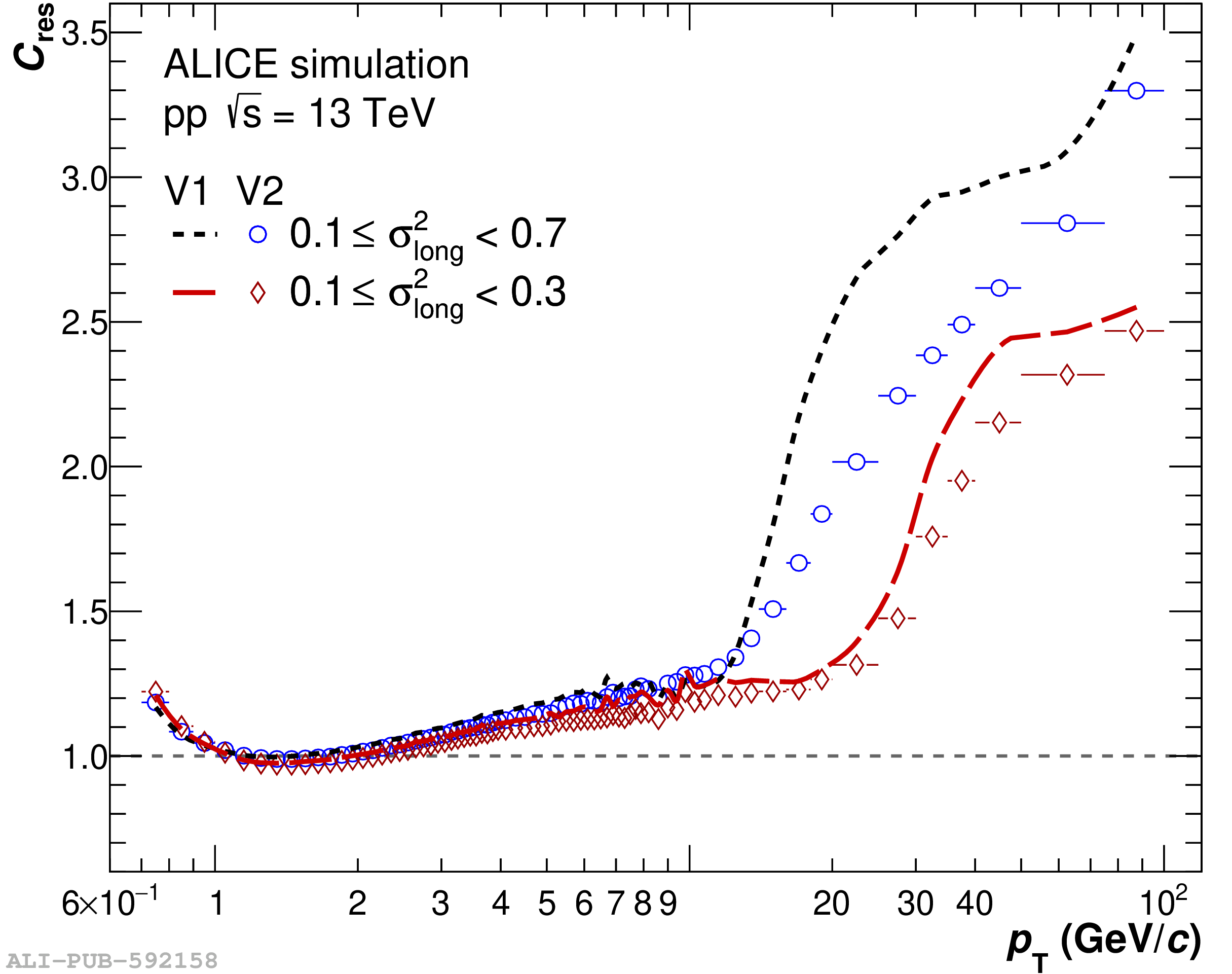  |
Figure 73
Illustration of the parameter-space of the photon $p_{\rm T}^{\rm iso}$ and $\sigma_{\rm long}^{2}$, used to estimate the background yield in the signal region ($\mathbb{A}$) from the observed yields in the three control regions ($\mathbb{B}$, $\mathbb{C}$, $\mathbb{D}$). The red regions indicate areas dominated by background and the blue regions by the photon signal. The color gradient indicates mixture of signal and background. | 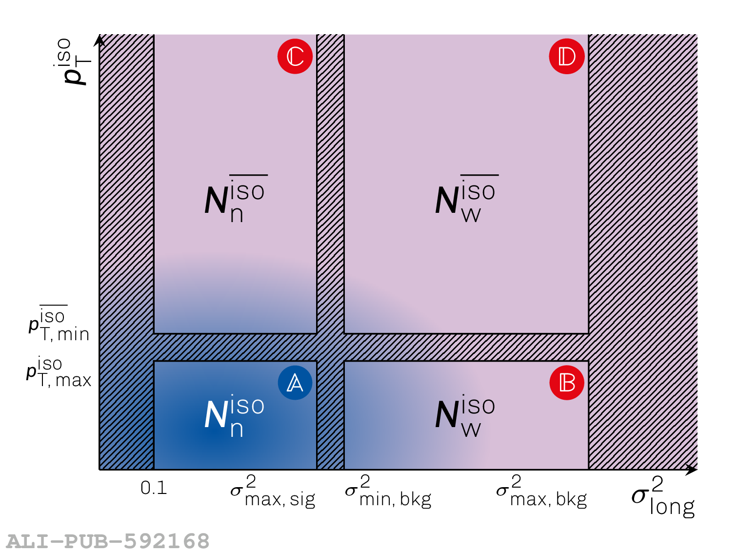 |


Figure 75
Isolated photon corrected purity in pp collisions at $\sqrt{s}=$ 7 TeV with $\pt^{\rm iso}< $ 2 GeV/$c$ and $|\eta^{\gamma}| < $ 0.27 calculated using Eq. 35, taken from [50] (left) and for pp and p$-$Pb collisions at $\sqrt{s_{\rm NN}}=$ 5.02 TeV with $|\eta^{\gamma}| < $ 0.67 using the template fit technique taken from [51] (right). The boxes indicate the systematic uncertainty, while the error bars reflect the statistical uncertainty. Figures are taken from the mentioned references. | 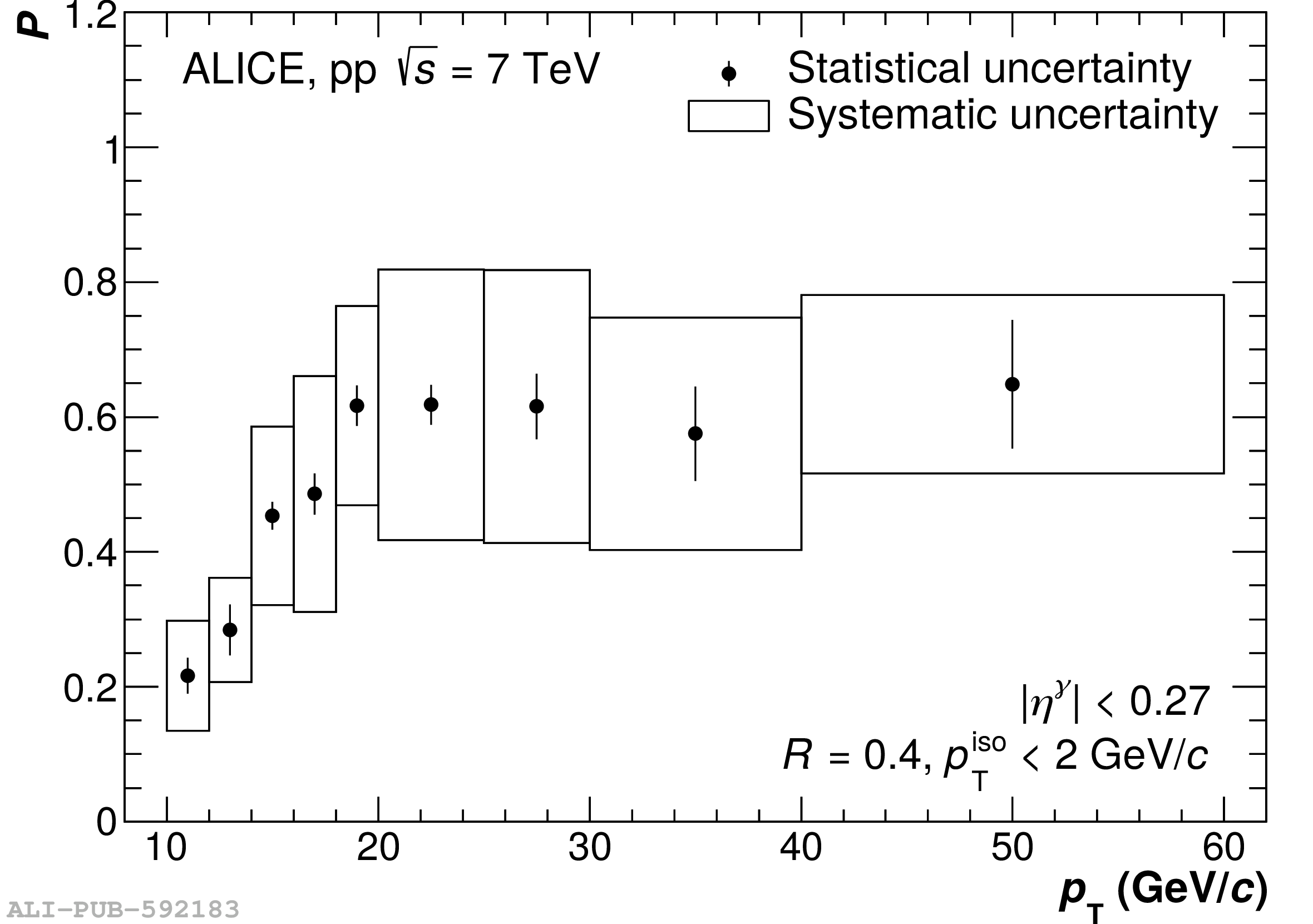 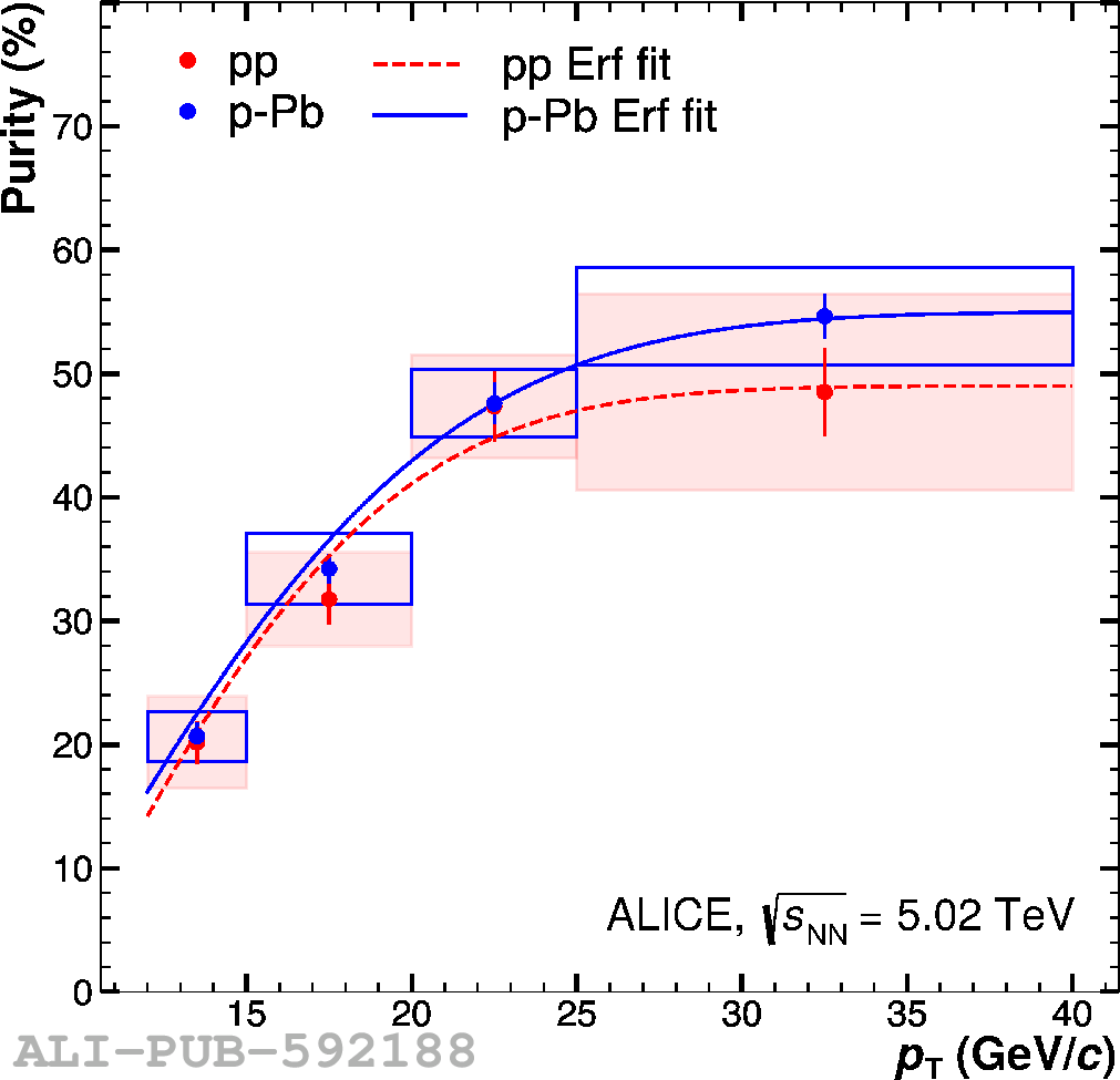 |
Figure 76
Invariant mass distribution for neutral pion and $\eta$ meson candidates at intermediate (left) and high (right) transverse momenta reconstructed with both photons in the EMCal in pp collisions at $\sqrt{s}=$ 13 TeV using the EMCal L1 trigger sample. The combinatorial background is described using the rotation background technique. For the higher $p_{\rm T}$ slice only the $\eta$ meson invariant mass window is shown as the $\pi^{0}$ meson cannot be reconstructed using the EMC invariant mass technique at these momenta. | 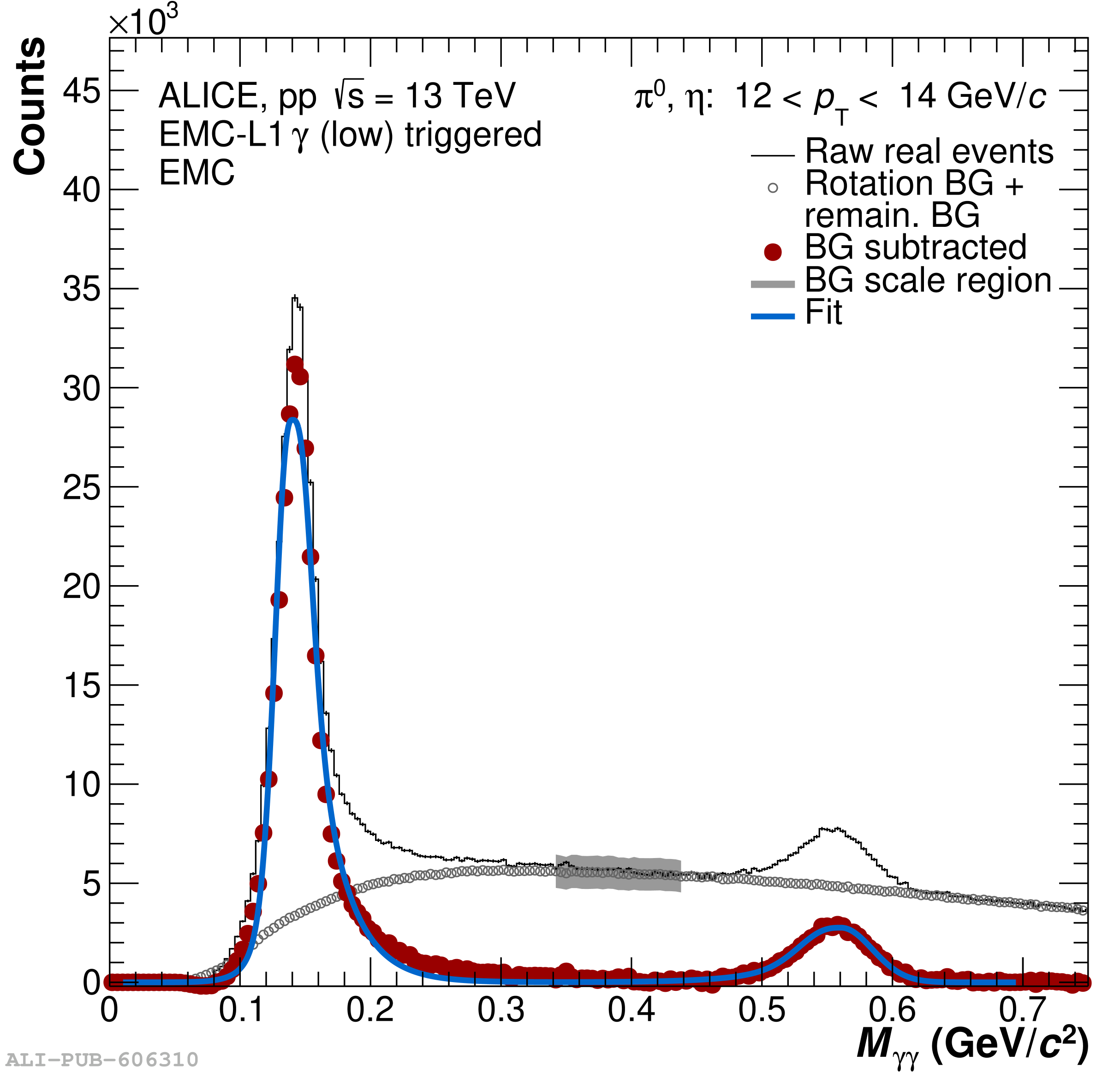 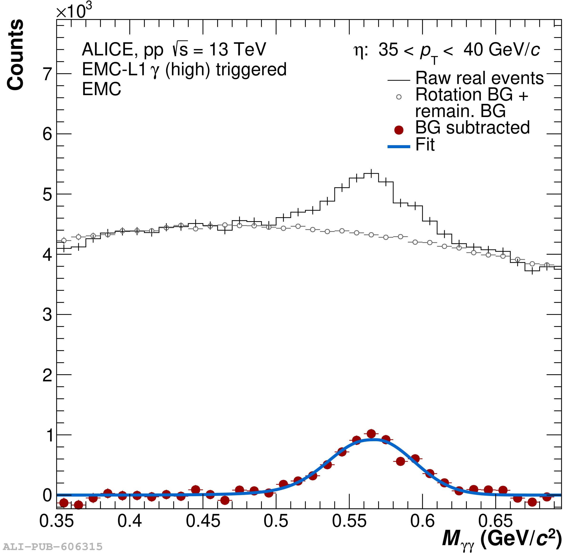 |
Figure 77
Invariant mass distribution for neutral pion candidates at low (left) and high (right) transverse momenta reconstructed using the PCM-EMC technique in pp collisions at$\sqrt{s}=$ 13 TeV using the minimum bias and EMCal L1 trigger sample. The combinatorial background is described using the mixed-event background technique. | 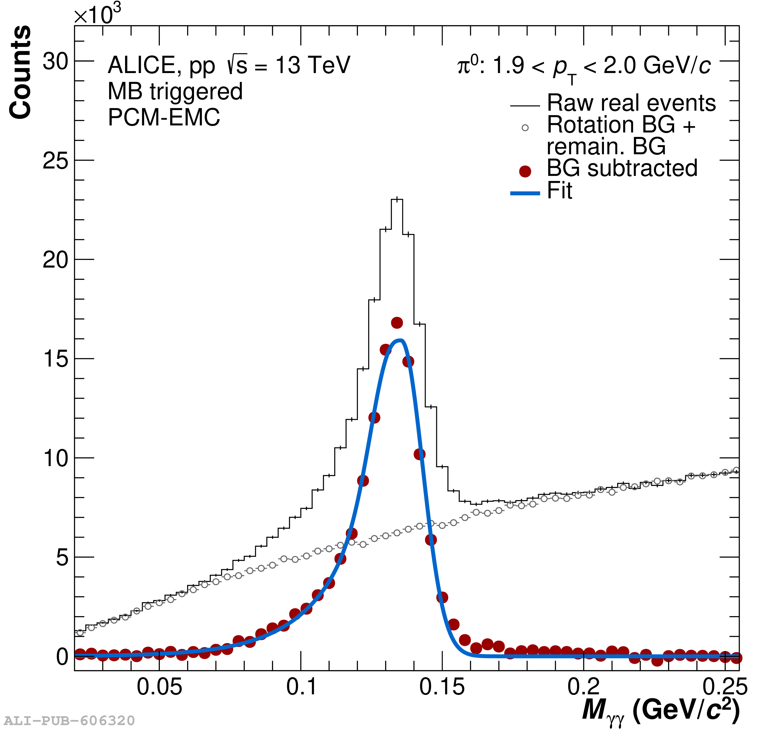 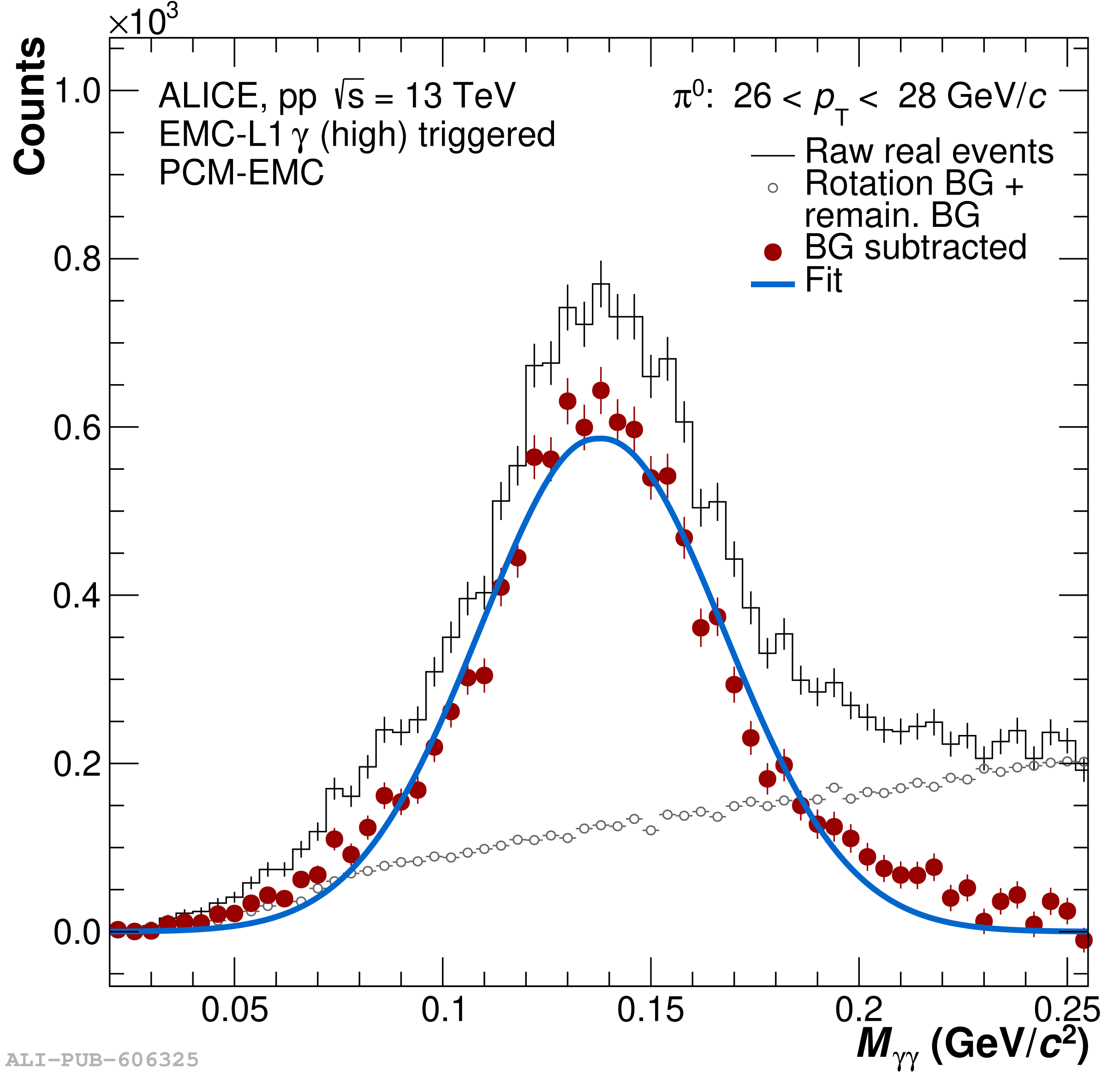 |
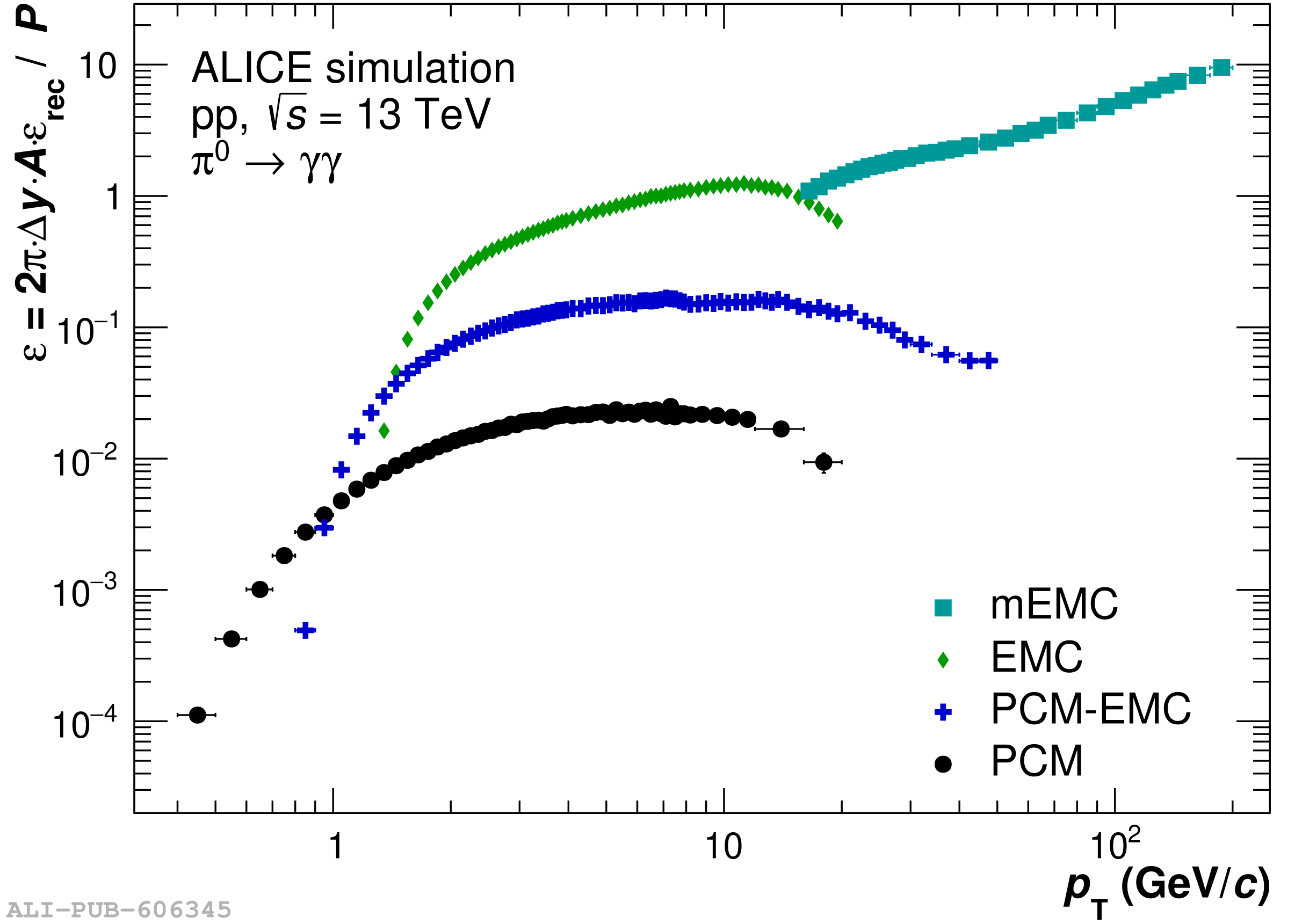
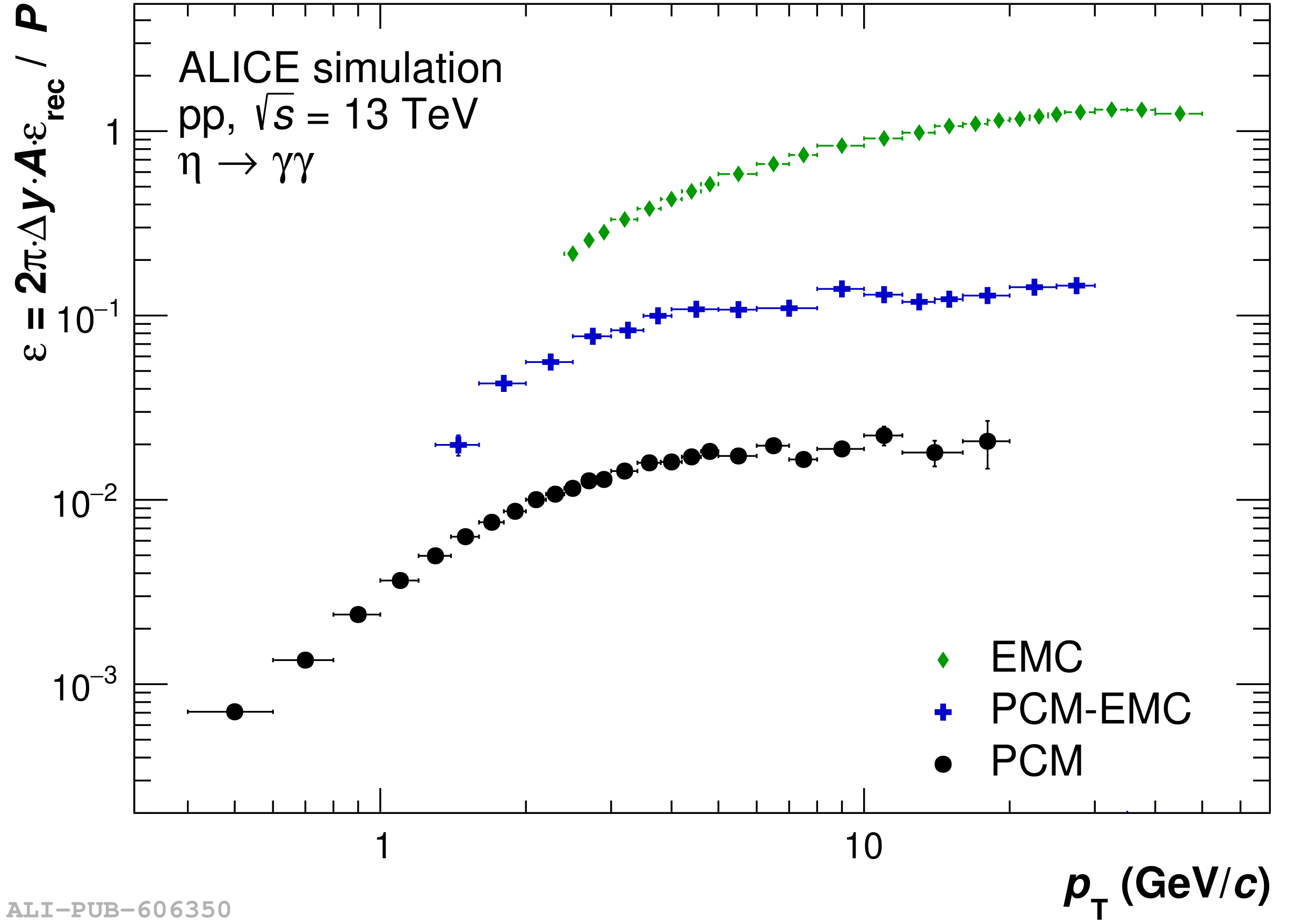
Figure 81
Invariant mass distribution for neutral pion candidates at intermediate (left) and high (right) transverse momenta reconstructed with both photons in the EMCal for pp and Pb$-$Pb collisions in different centrality classes at $\sqrt{s_{\rm NN}}=$ 5.02 TeV The distributions are normalized to the integral in the displayed invariant mass region to be able to compare the shapes of the invariant mass distributions and their difference in the signal-to-background ratio. The gray vertical line indicates the nominal pion mass, while vertical black and red lines indicate the reconstructed neutral pion mass in pp and central Pb$-$Pb collisions, respectively. | 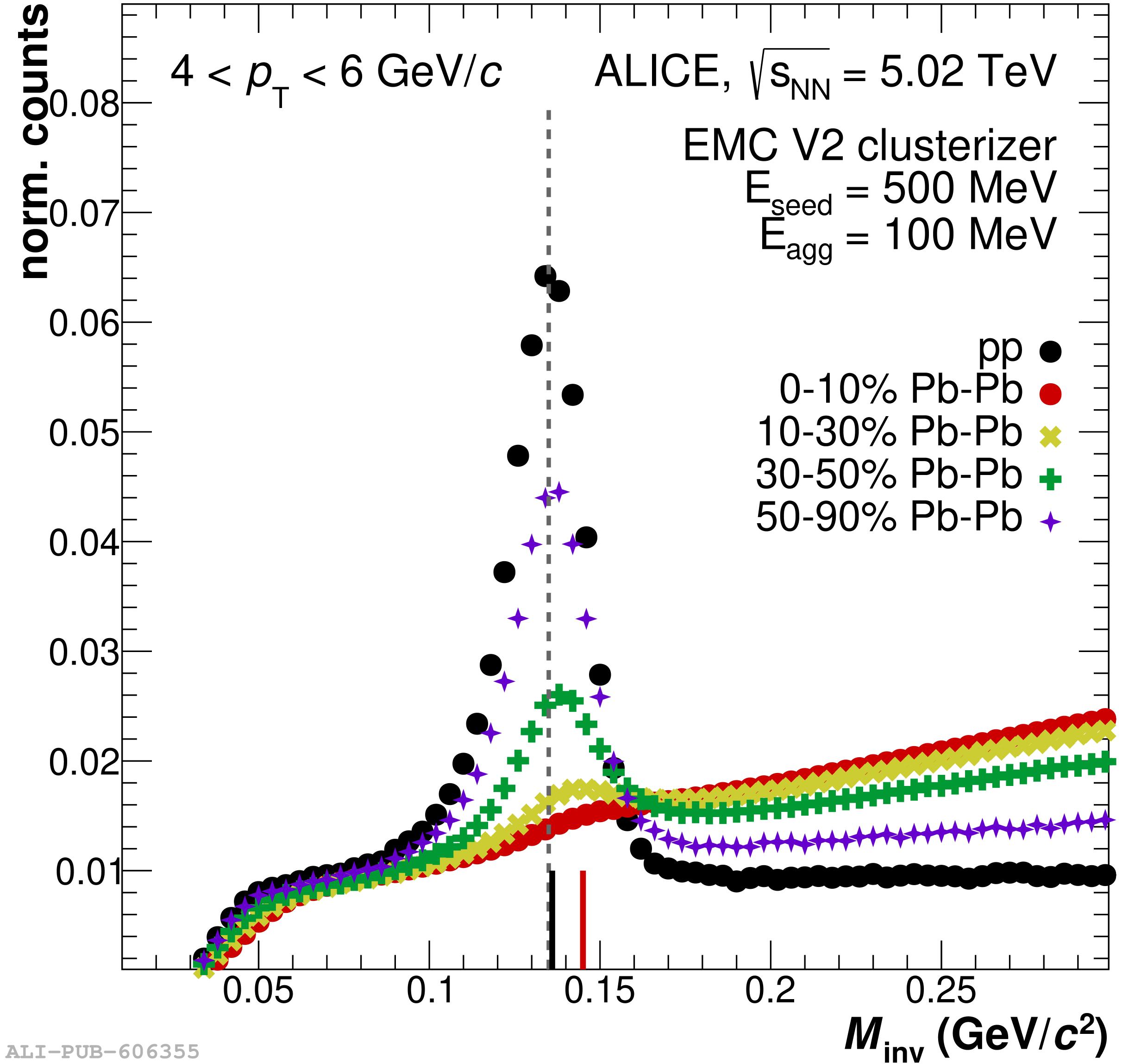 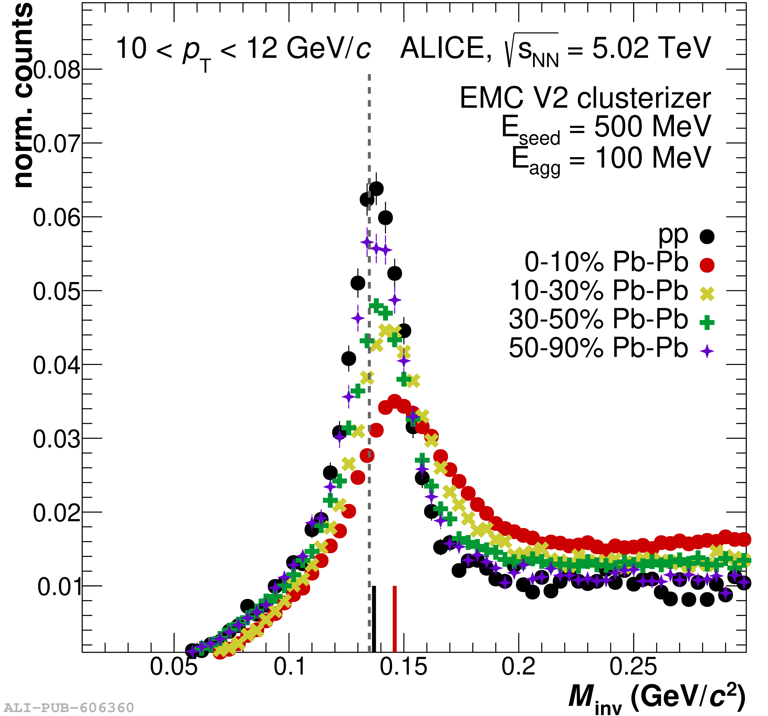 |
Figure 83
Left: Decomposition of the $\sigma_{\rm long}^{2}$ distribution at 90 $ < p_{\rm T} < $ 100 GeV/$c$ in its contributions from neutral pions reconstructed with both photons in one cluster (full black dots) or only one photon (open black dots) based on PYTHIA8 di-jet simulations. Additionally, the contributions from $\eta$ mesons (open blue dots), direct photons (orange histogram), primary electrons (green histogram) and other hadrons (blue histogram) are displayed. Right: Comparison of the $\sigma_{\rm long}^{2}$ distribution between data (black) and simulation (red). | 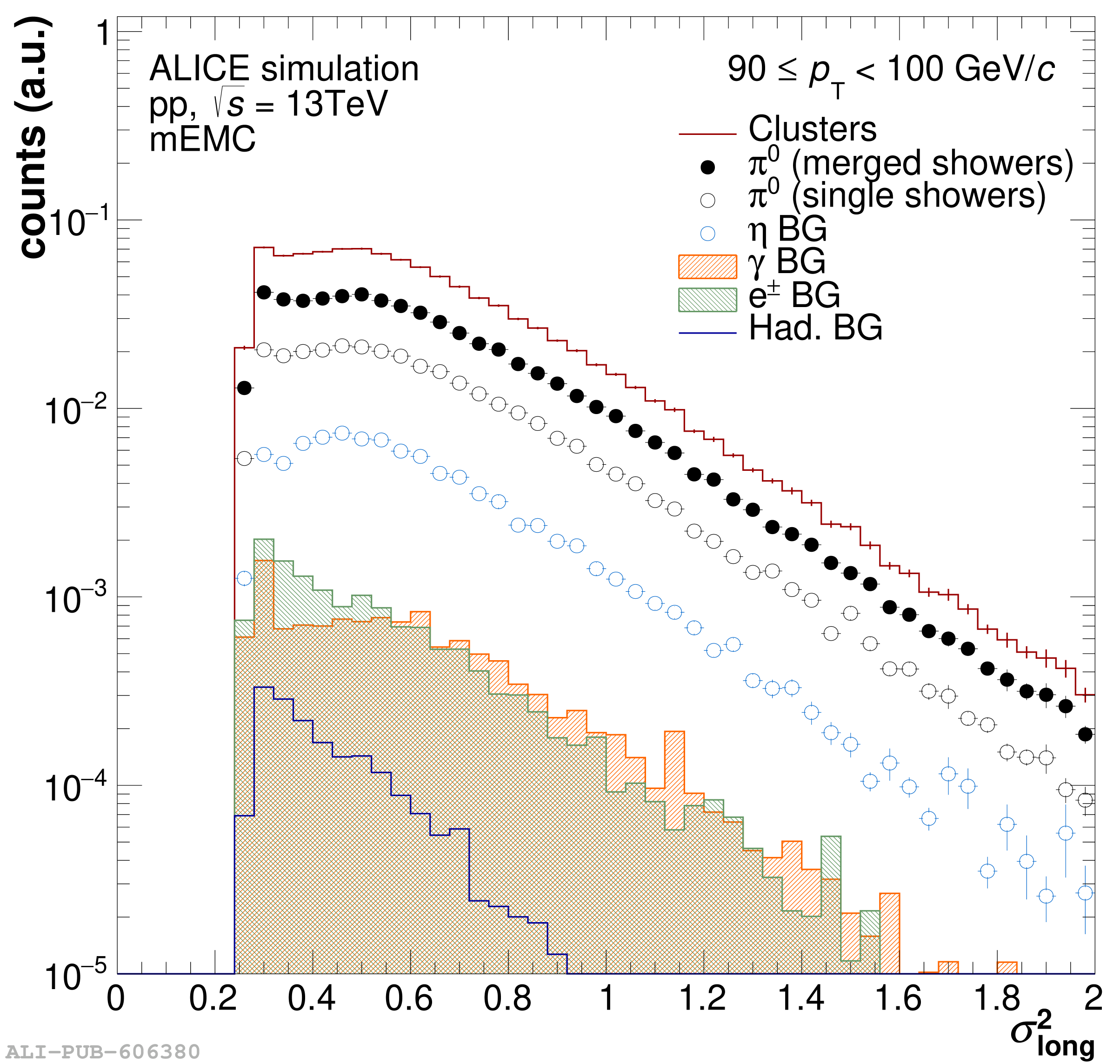 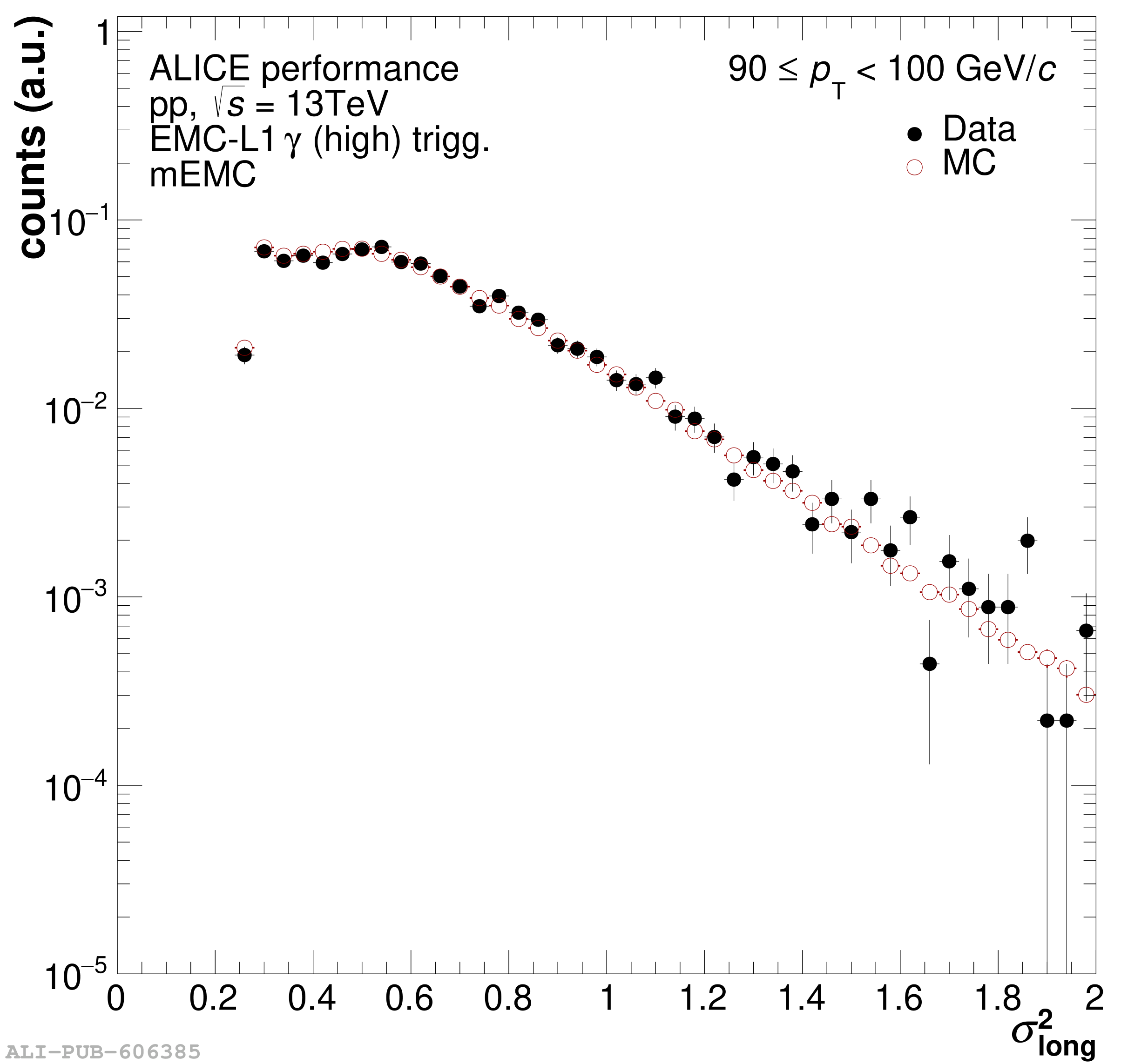 |
Figure 84
Left: Contamination ($c_i$) of the neutral pion candidate sample split into the different contributions according to the PYTHIA8 di-jet simulations. Right: Purity of the neutral pion candidate sample without modifications (blue dots) and after additional corrections to adjust the simulation to the measured $\eta$ meson, expected direct photon and heavy-flavor-electron contributions (red open dots). | 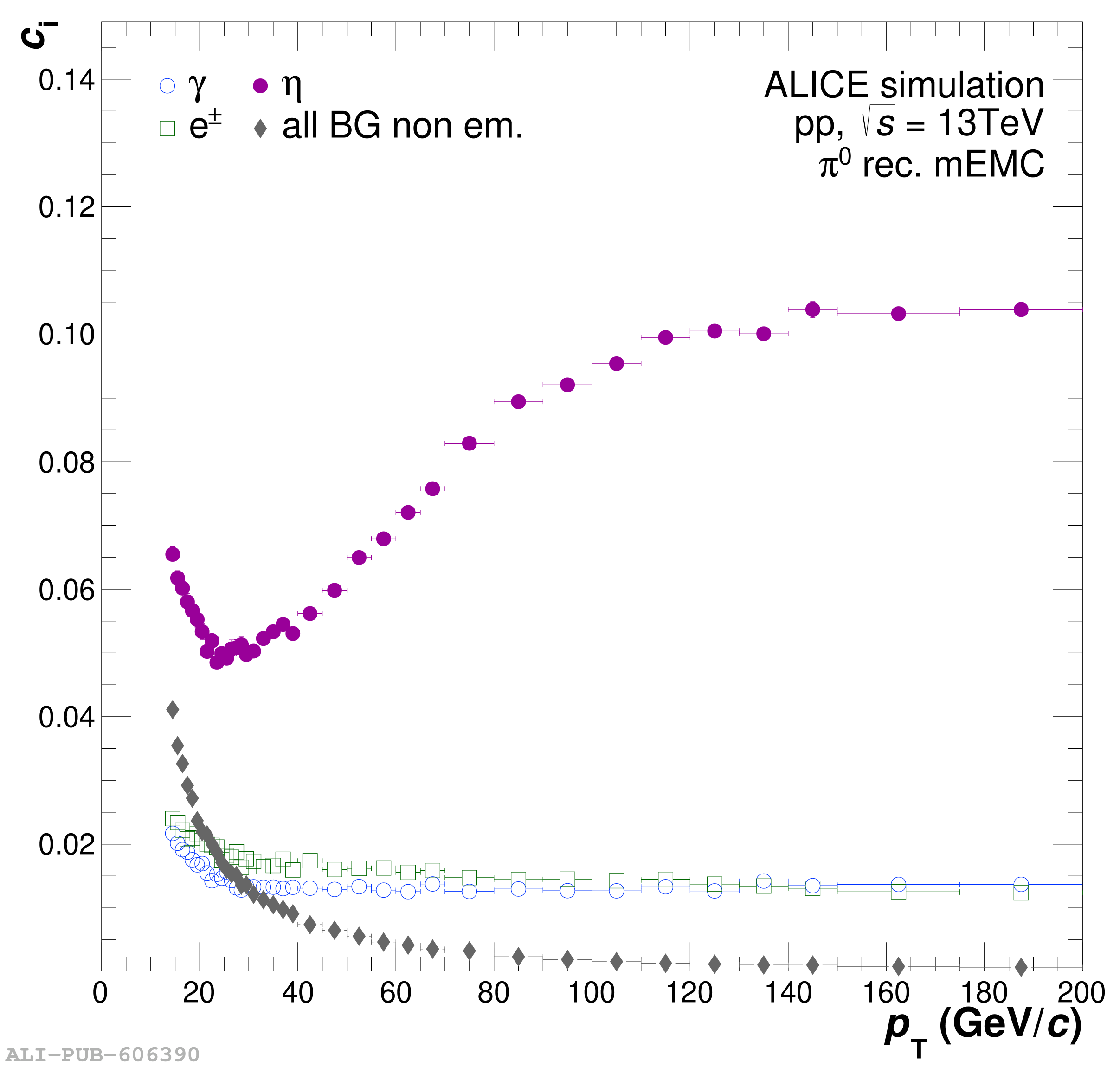 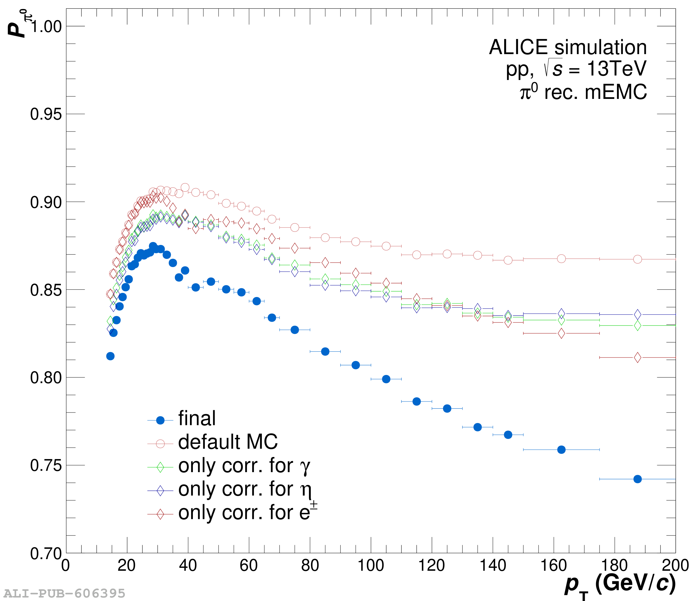 |
Figure 85
a) Mean cluster energy shift versus transverse momentum for three different neutral pion merged cluster types from PYTHIA8 simulations with two jets in the final state at $\sqrt{s}=$ 13 TeV. Clusters with no overlapping particles within $R< $0.05 around the momentum vector of the $\pi^0$ on Monte Carlo generator level are shown in red, while clusters with 1$-$2 overlapping particles are shown in green and clusters with more than two overlapping particles in blue. An increasing overlap of particles shifts the cluster energies to larger values. b) Fractions of clusters from the three overlap types in the total cluster sample are shown in the same colors. The bands indicate the systematic variations on the fractions, which are applied in the toy simulation in order to obtain the final systematic uncertainty shown in the shaded gray band versus transverse momentum. | 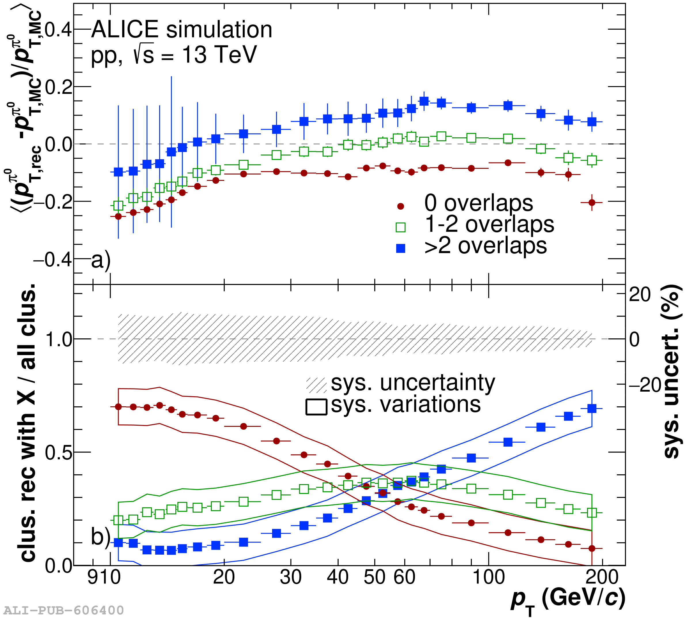 |
Figure 86
Left: Mass of split clusters for pp collisions at $\sqrt{s}=$ 13 TeV for the V1 clusterizer with two local maxima compared to the invariant mass distribution obtained from pairs of V2 clusters for the neutral pion. Right: Mass of split clusters for pp and Pb$-$Pb collisions in different centrality classes at $\sqrt{s_{\rm NN}}=$ 5.02 TeV. For the Pb$-$Pb comparison plot, the distributions are normalized to the maximum in the peak region to be able to compare the shapes of the invariant mass distributions. The gray vertical line indicates the nominal pion mass. | 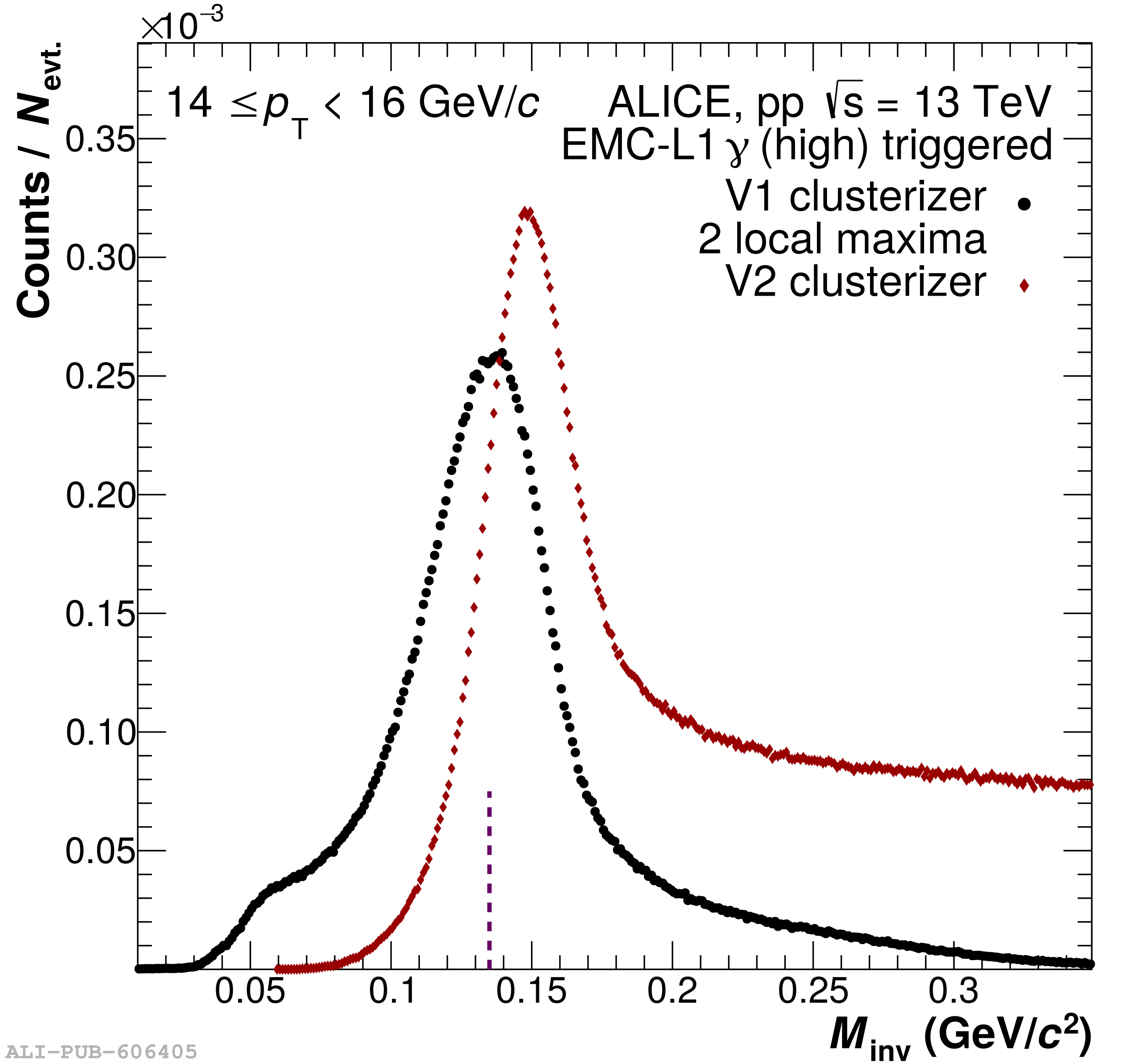 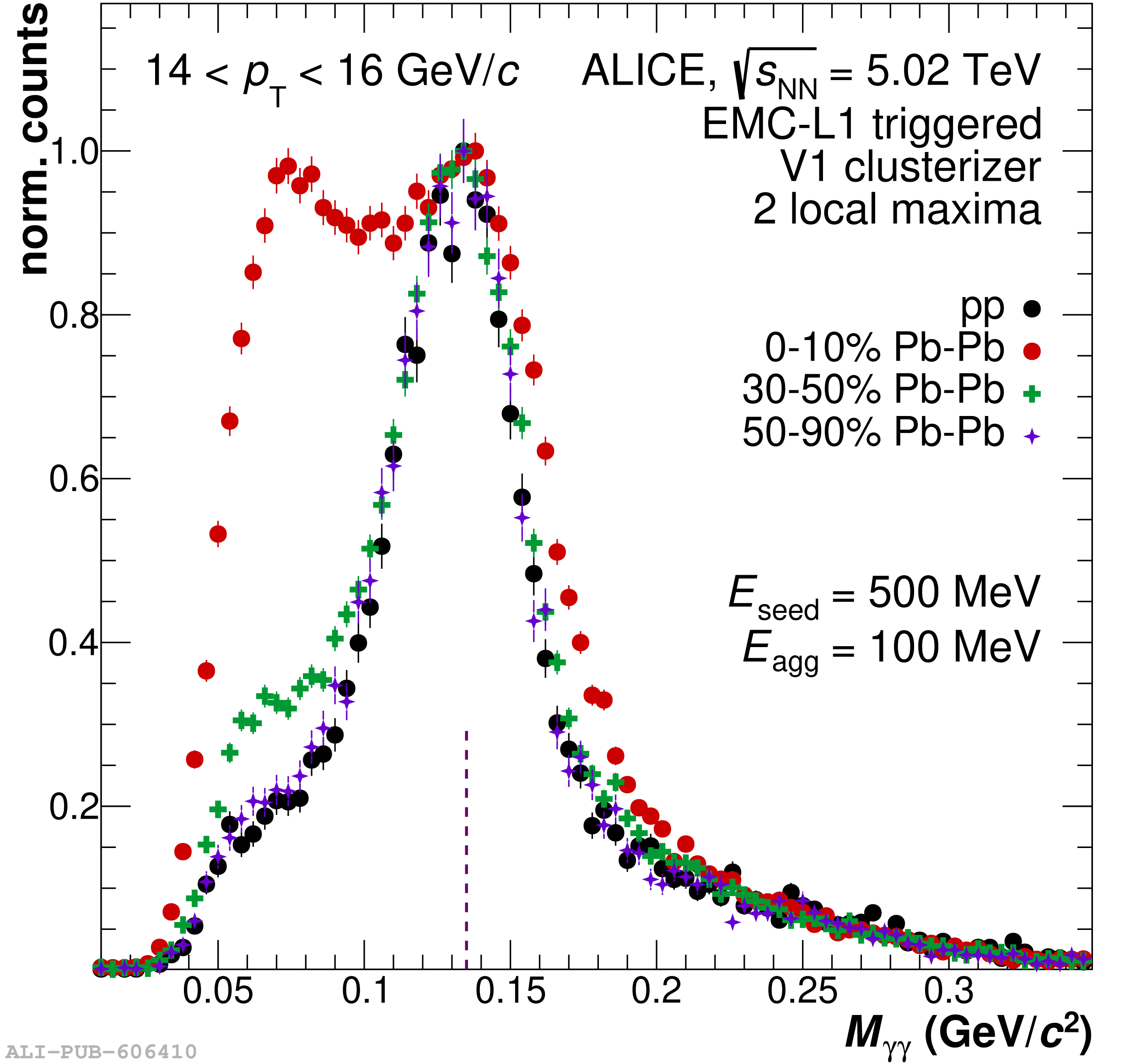 |
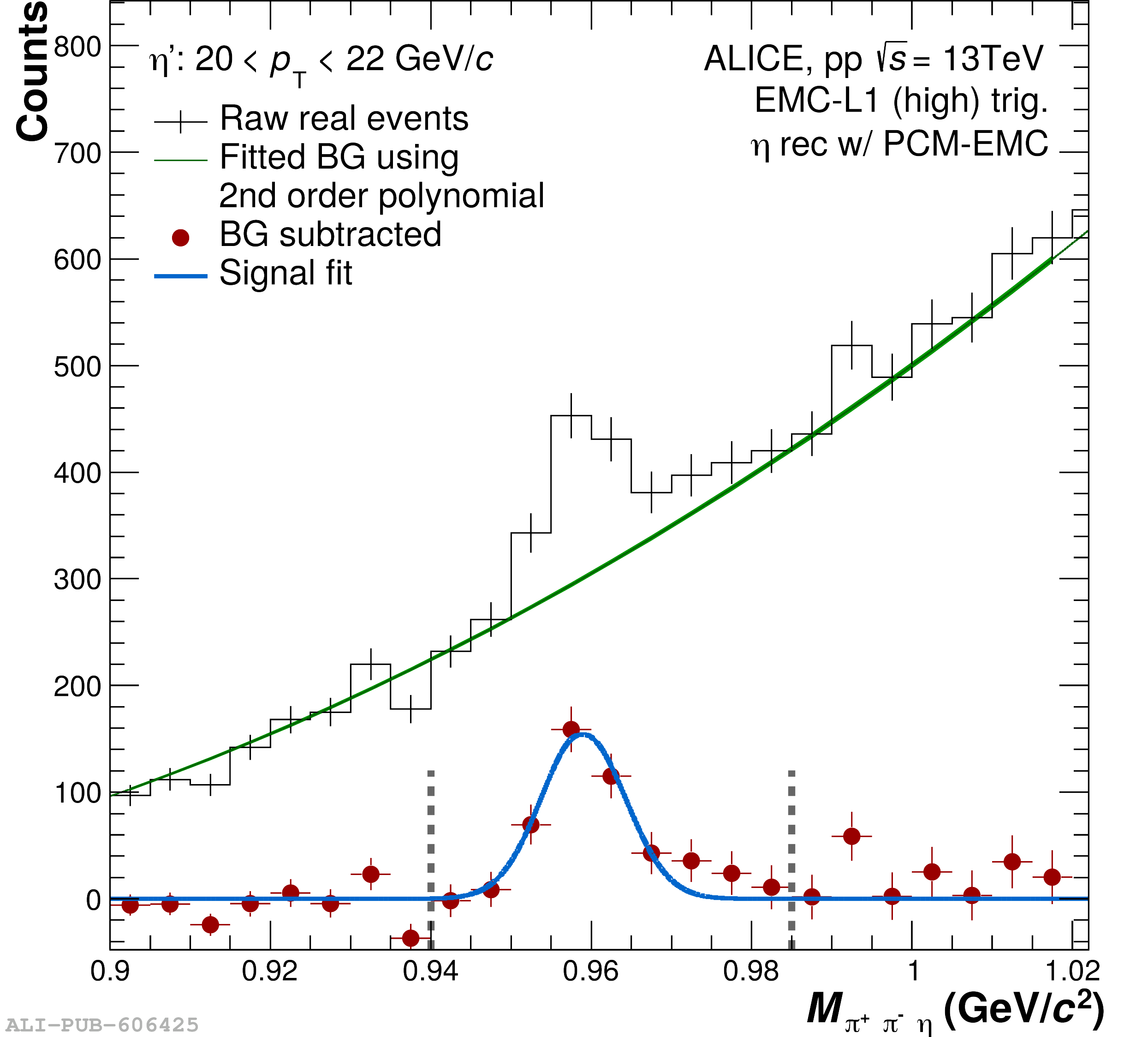
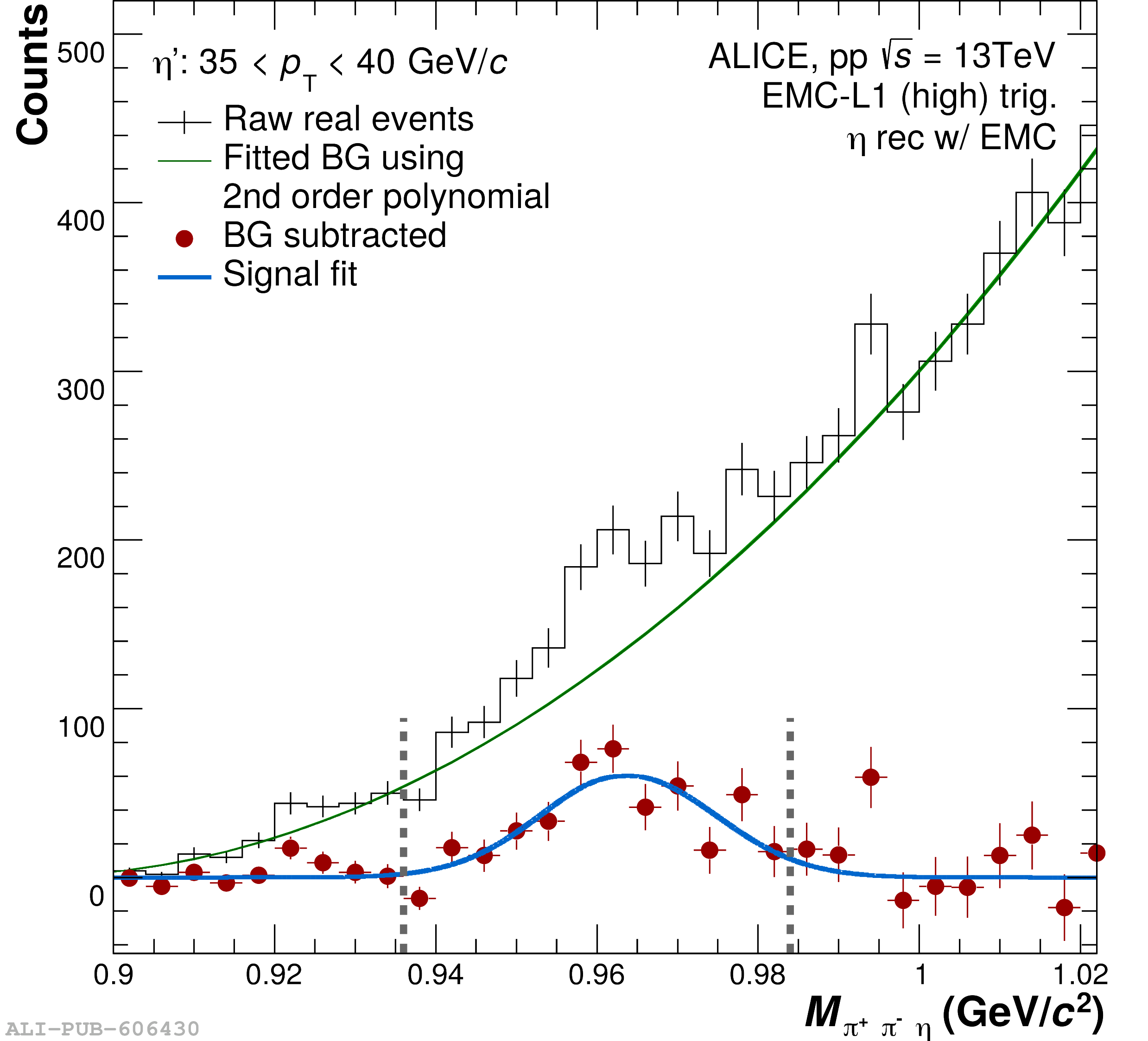
Figure 90
$n\sigma^{\textrm{TPC}}_{e^\pm}$ distribution without (black) and with (green) EMCal electron identification cuts of $E/p$ and $\sigma_{\rm long}^{2}$. Electrons form a Gaussian distribution centered around zero, indicated by the gray dashed line. The signal and background selection windows considered for the following $E/p$ plots are indicated by the red and blue shaded area, respectively. The distributions are shown for various event triggers in pp collisions at $\sqrt{s}=$ 13 TeV in different $p_{\rm T}$ intervals. | 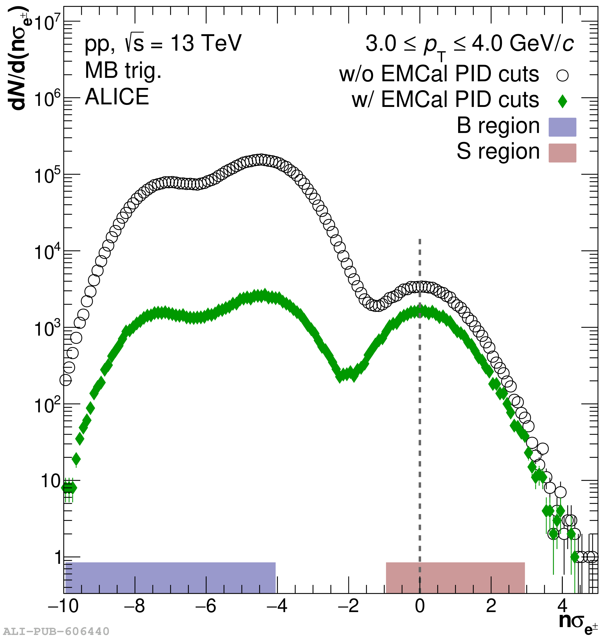 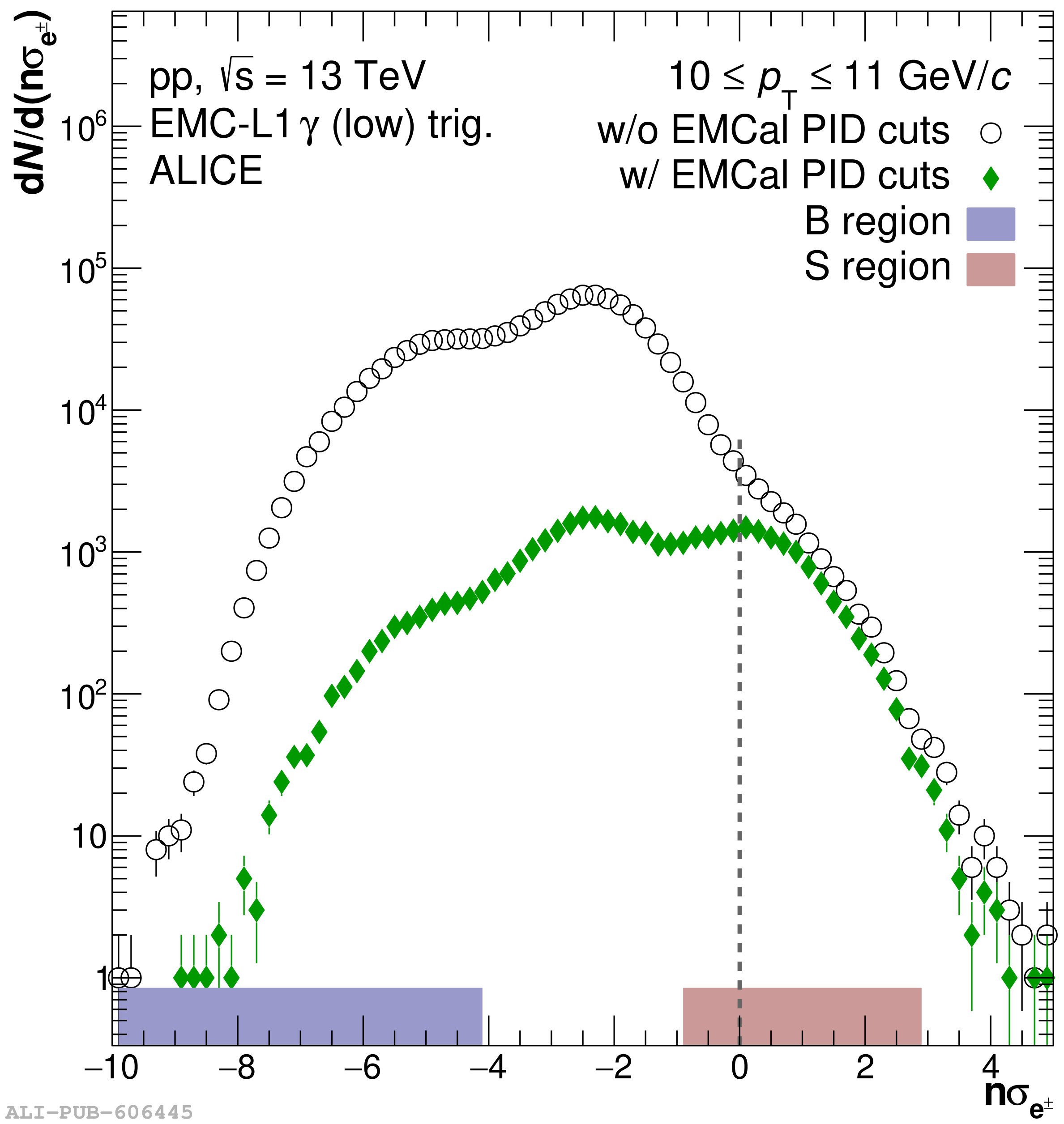 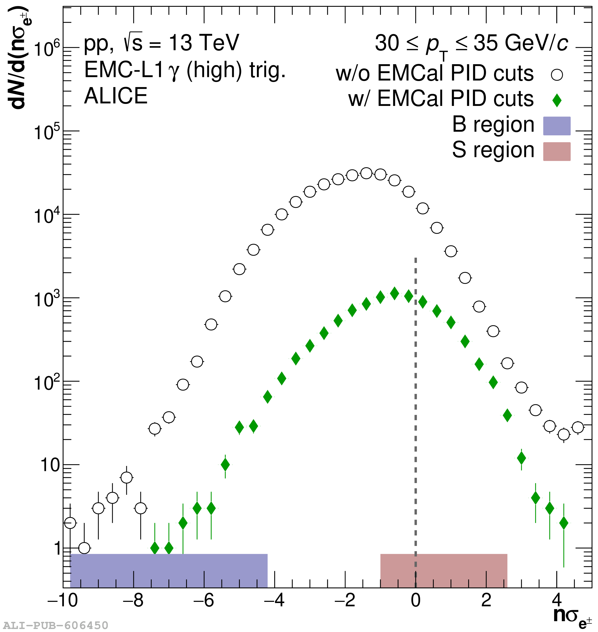 |
Figure 91
$E/p$ distribution for electron candidates selected by applying $-1 \leq n\sigma^{\textrm{TPC}}_{e^\pm} \leq 3$ (black open circles), and for hadrons with $-10 \leq n\sigma^{\textrm{TPC}}_{e^\pm} \leq -4$ (blue dots) scaled to match the electron distribution in the range indicated by the blue shaded box. The red diamonds reflect the remaining signal distribution after background subtraction and the corresponding signal fit using a Gaussian with an exponential tail is overlaid in dark red. The distributions are shown for various event triggers in pp collisions at $\sqrt{s}=$ 13 TeV in different$p_{\rm T}$ intervals. | 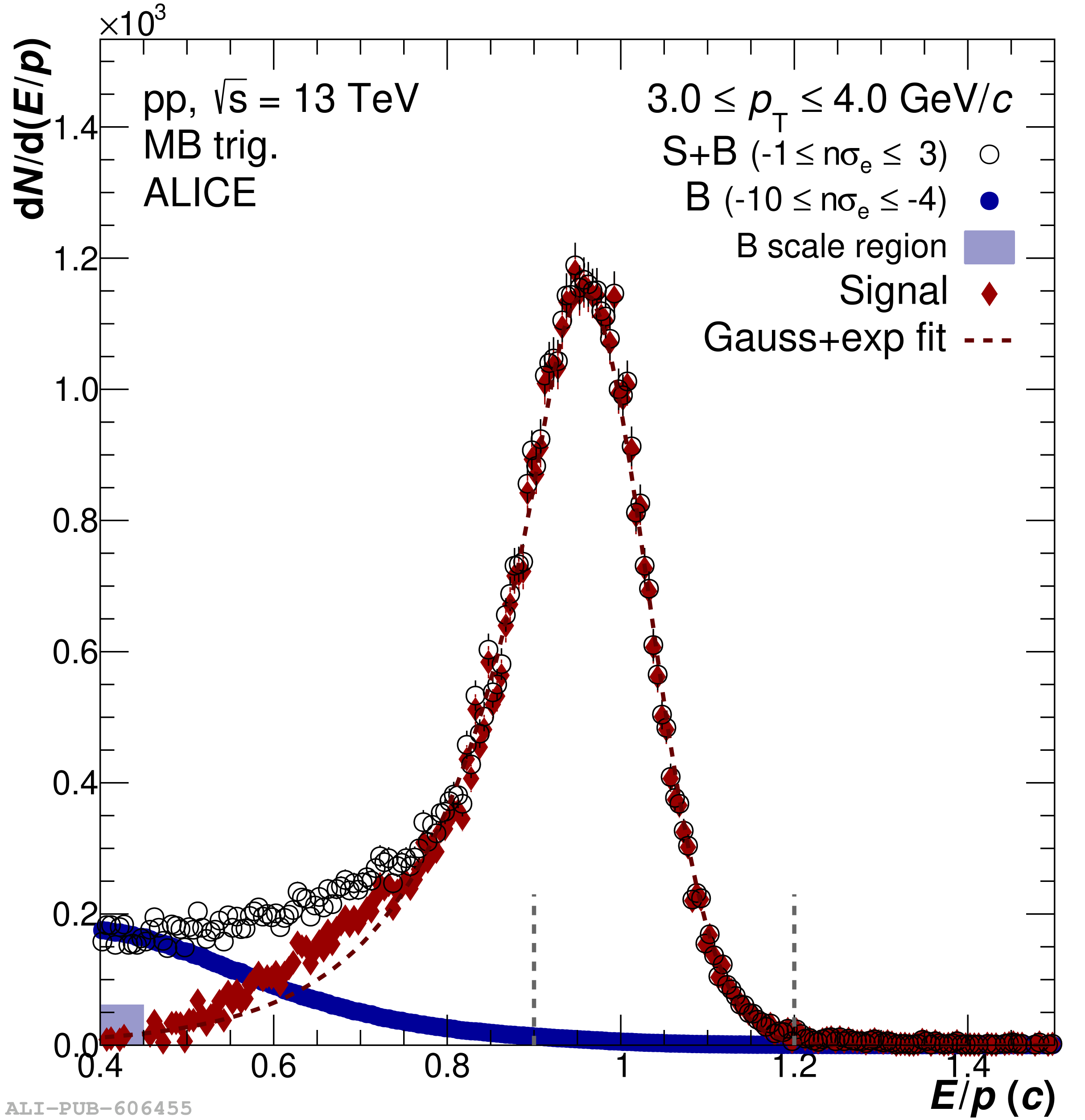 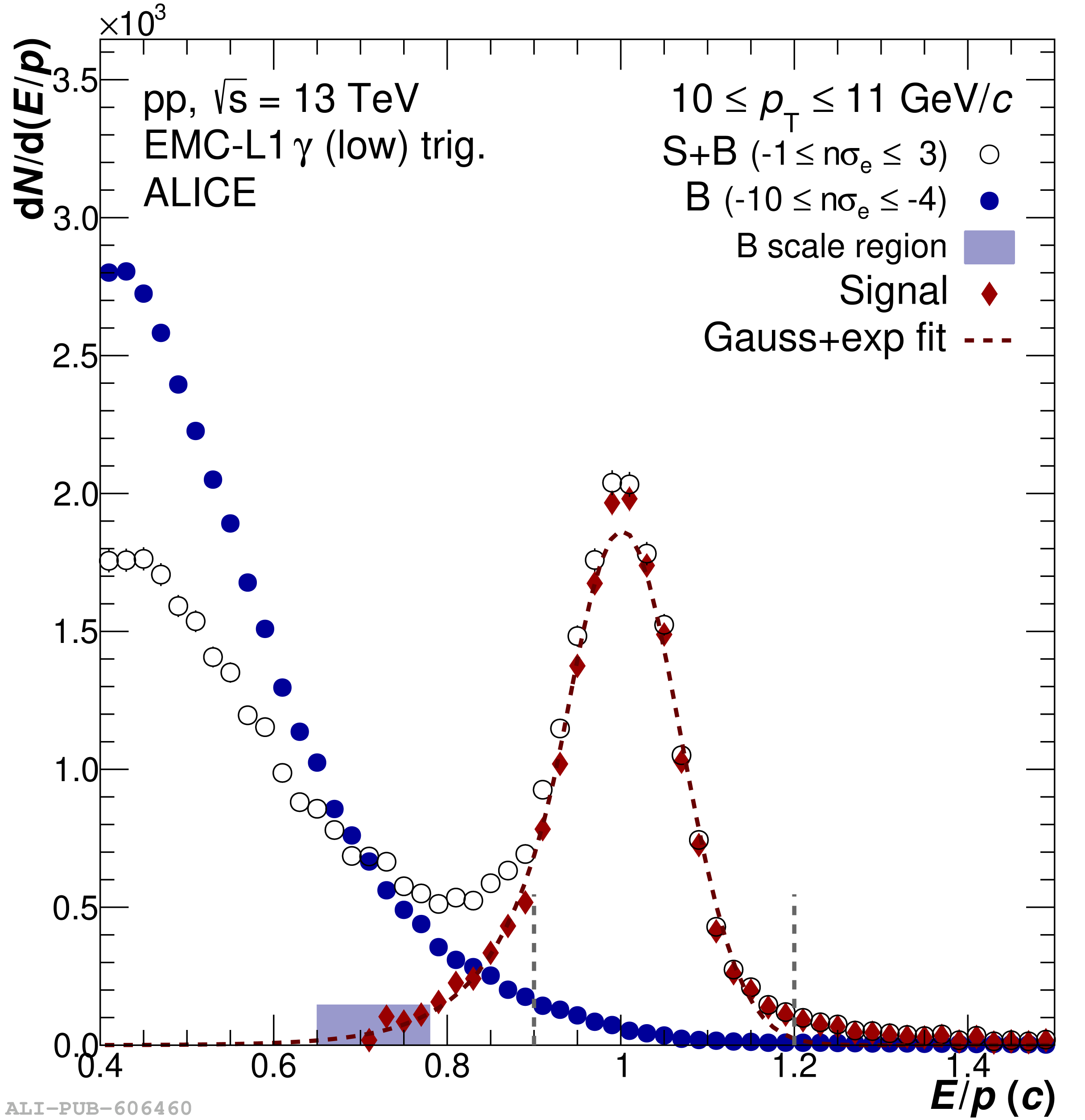 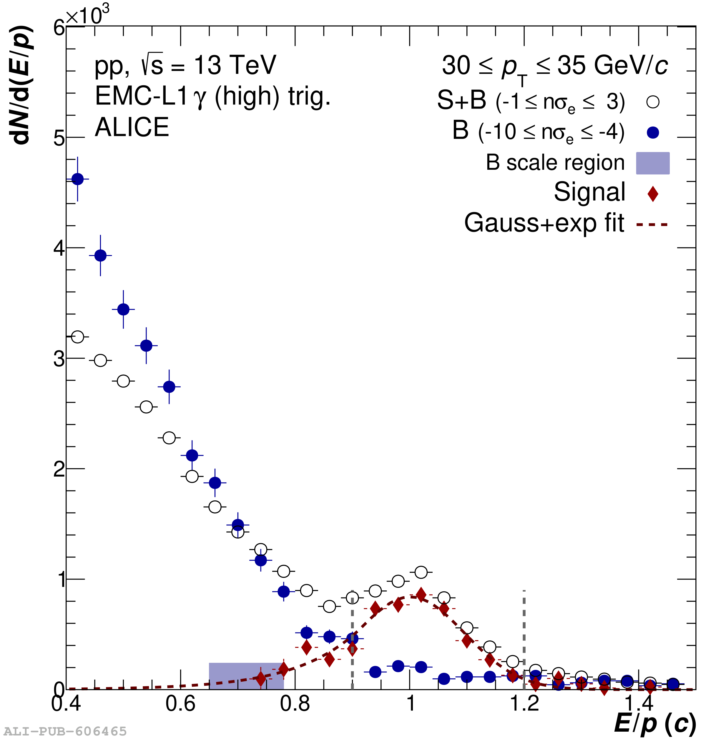 |
Figure 92
Left: Comparison of the $E/p$ distribution between real (black) and simulated (red) data for electron candidates with 3 $< p_{\rm T}< $ 4 GeV/$c$ in pp collisions at $\sqrt{s}=$ 13 TeV. Gaussian fits with exponential tails to both sides are superimposed for both distributions in the corresponding color. The truncated means for data and MC are indicated by vertical colored lines. The truncation and signal integration window is indicated by vertical dashed gray lines. Right: Data and simulation comparison of width (top) and mean (bottom) of the $E/p$ distributions of electrons as a function of transverse momentum in pp collisions at $\sqrt{s}=$ 13 TeV. Fit functions are shown as dashed lines, where their functional form is given in the respective legends. | 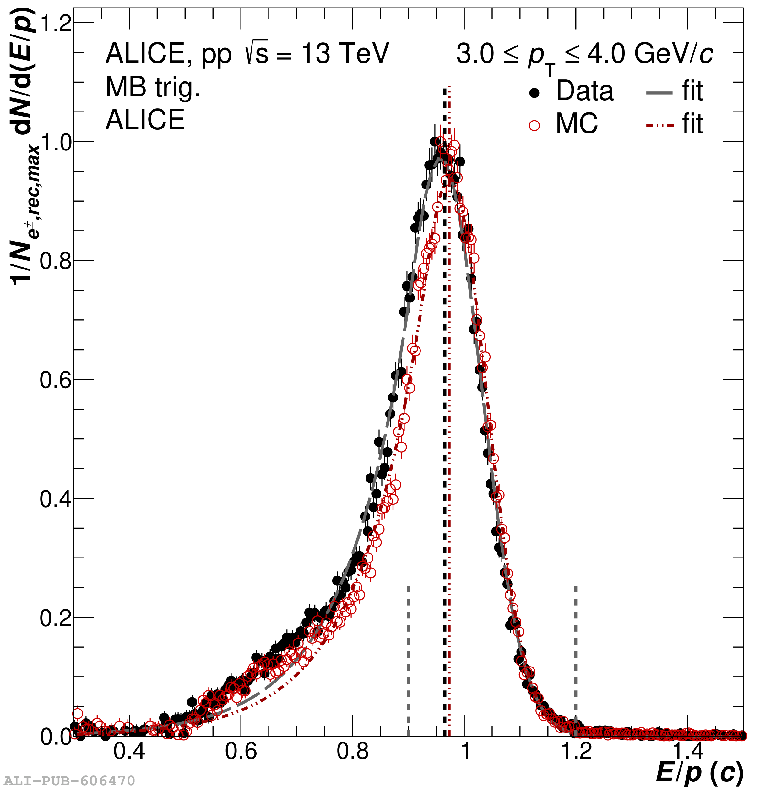 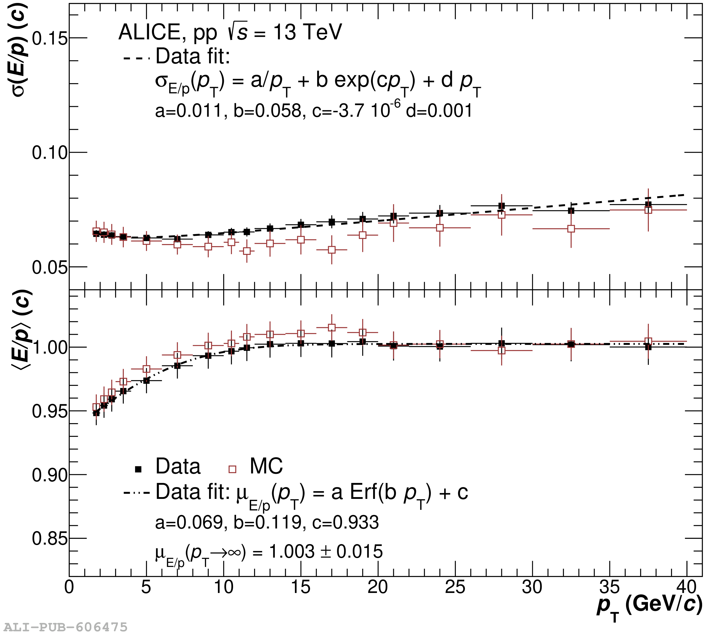 |
Figure 93
Data-driven purity ($P$) estimates of the electron sample after applying TPC and EMCal electron identification criteria as a function of $p_{\rm T}$ in pp collisions at $\sqrt{s}=$ 13 TeV (left) and in Pb$-$Pb collisions at $\sqrt{s_{\rm NN}}=$ 5.02 TeV (right). The boxes indicate the systematic uncertainty arising from the use of different scaling ranges for the hadronic background. | 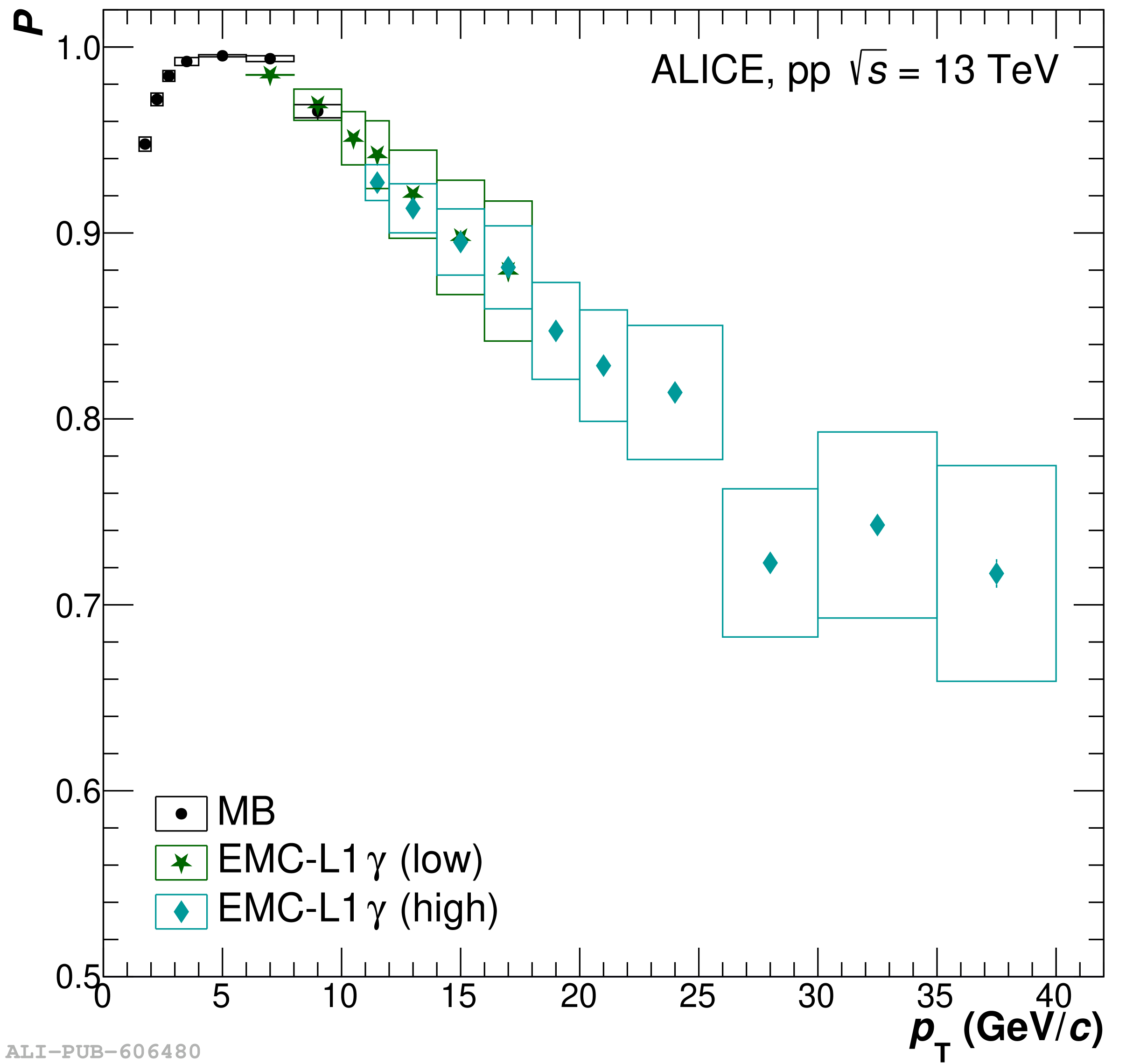 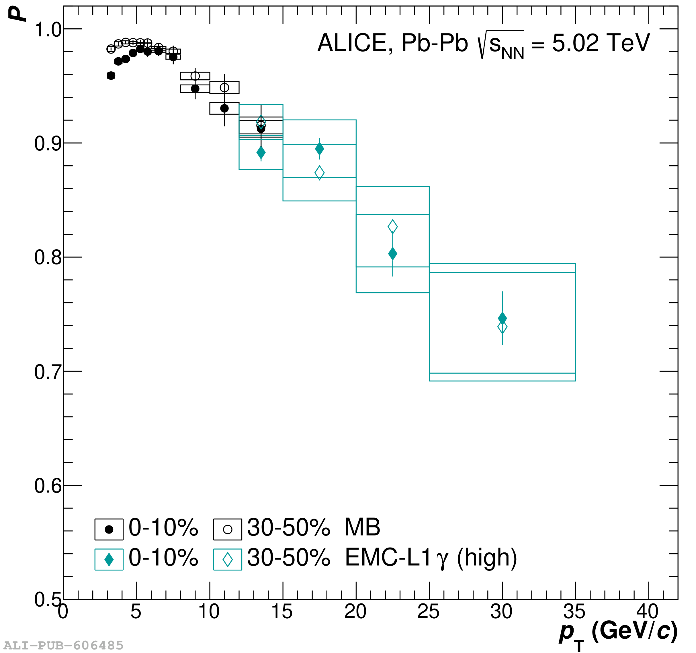 |
Figure 94
Invariant mass distribution of D*$^{+}$ candidates in pp collisions at $\sqrt{s}=$ 13 TeV for 65 $< p_{\rm T} < $ 80 GeV/$c$ (left) and 100 $< p_{\rm T}< $ 140 GeV/$c$ (right) using the EMCal L1 triggered data. The raw data distribution is shown in black, while the combined signal and background fit is overlayed as a blue line. The separated components of the signal and background contribution to the fit are displayed as red and gray lines, respectively. | 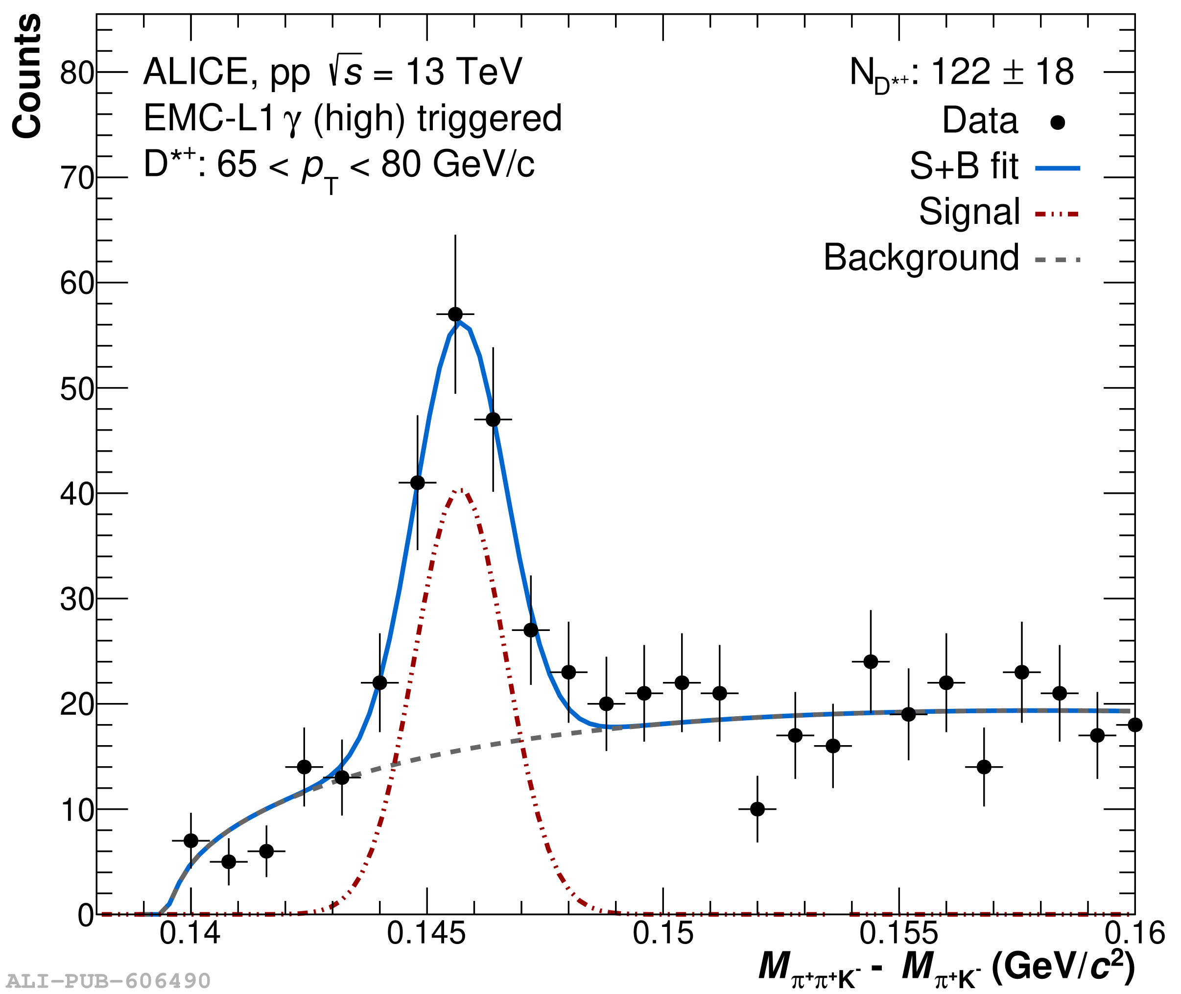 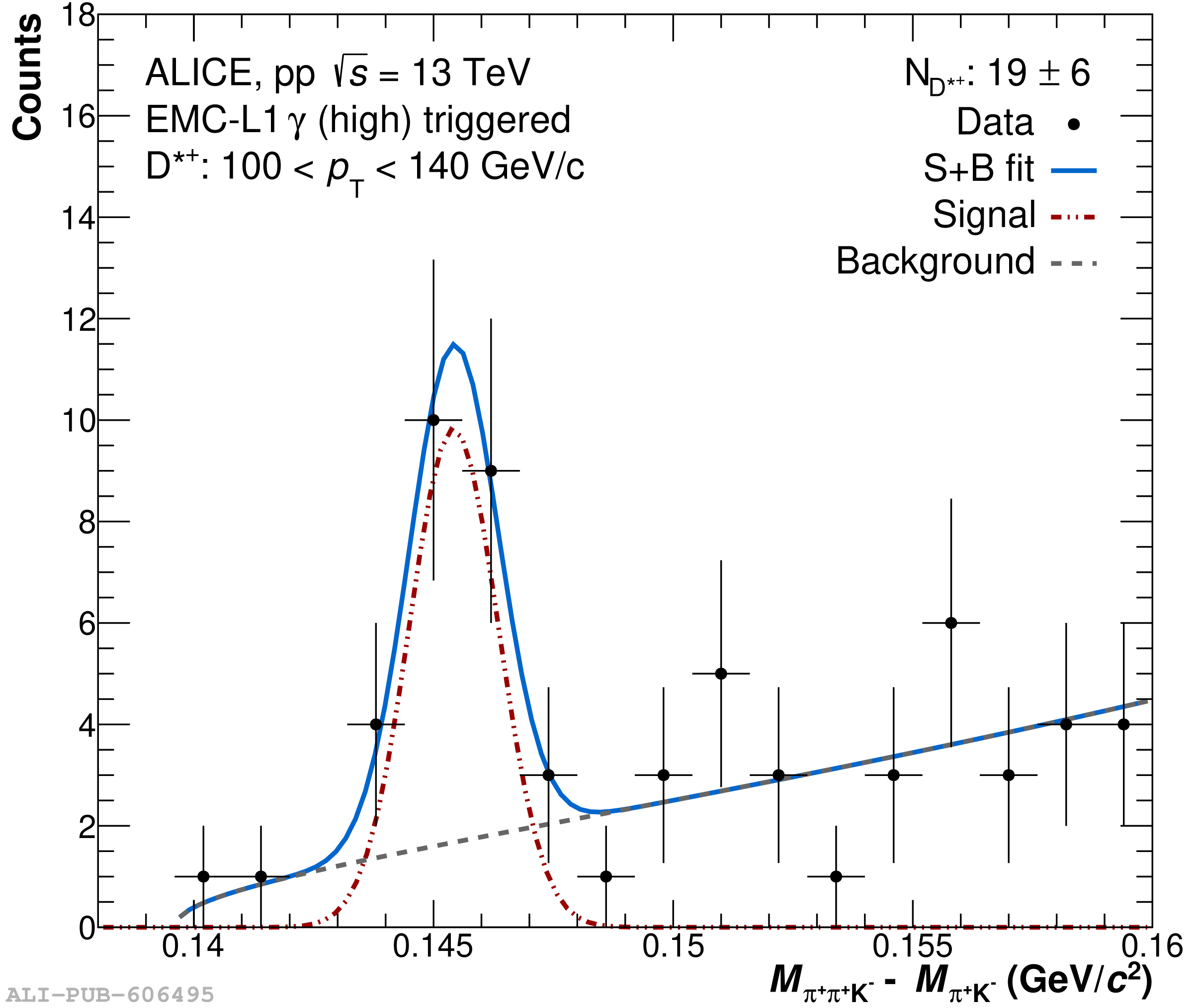 |
Figure 95
Invariant mass distribution of J/$\psi$ candidates in pp collisions at $\sqrt{s}=$ 13 TeV for 8 $< p_{\rm T}< $ 15 GeV/$c$ (left) and 30 $< p_{\rm T}< $ 40 GeV/$c$ (right). The gray open markers depict the distribution for e$^+$e$^-$ pairs where at least one track could be matched to an EMCal cluster. It is scaled by $1/2$ and $1/4$, respectively, for the different $p_{\rm T}$ intervals, to enhance the visibility. The black closed markers represent the distribution after applying the EMCal PID selections on at least one of the J/$\psi$ decay products. The combined signal and background fit is shown by the blue line, while the polynomial background and pure signal fit are shown as gray and red lines respectively [75]. | 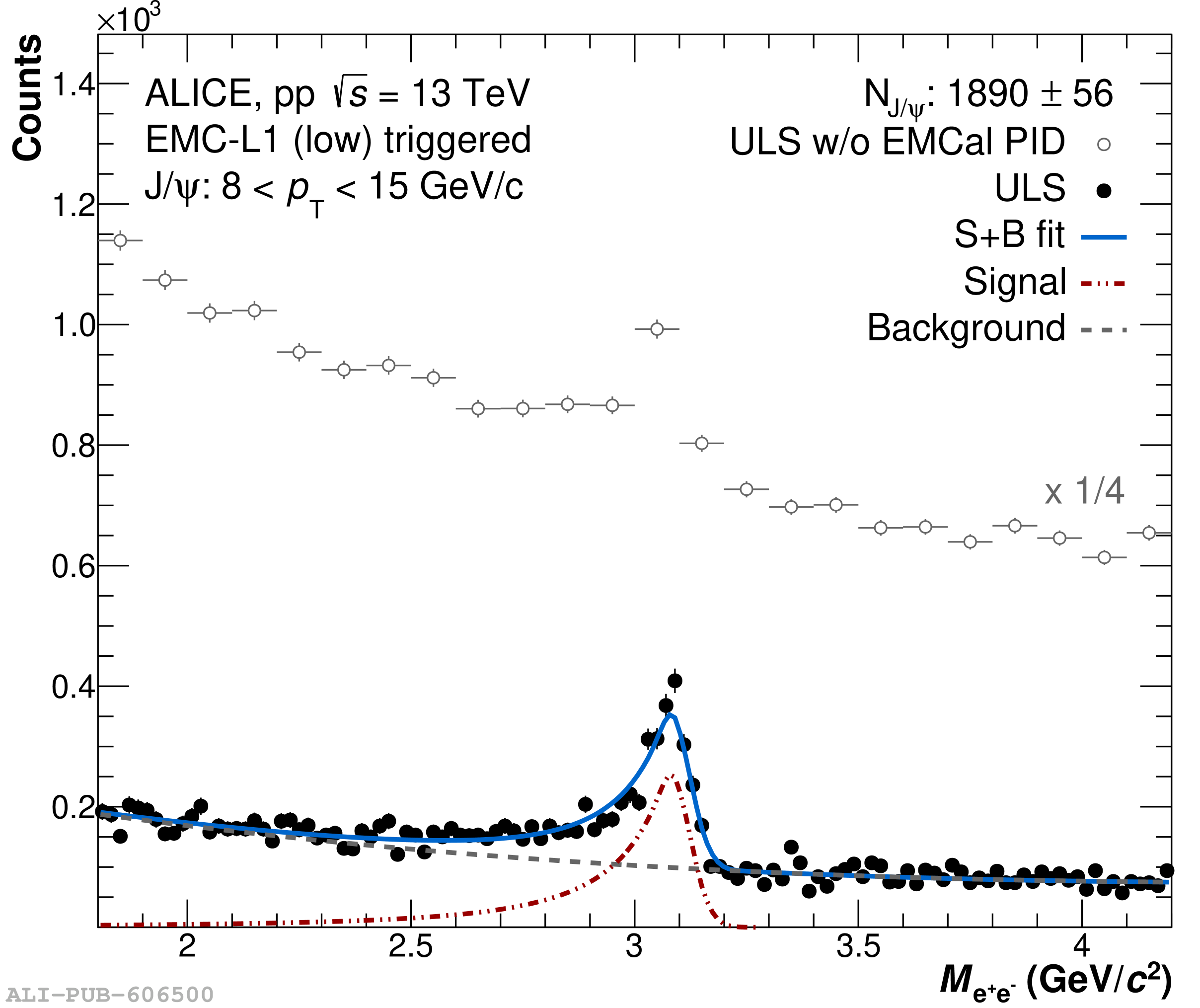 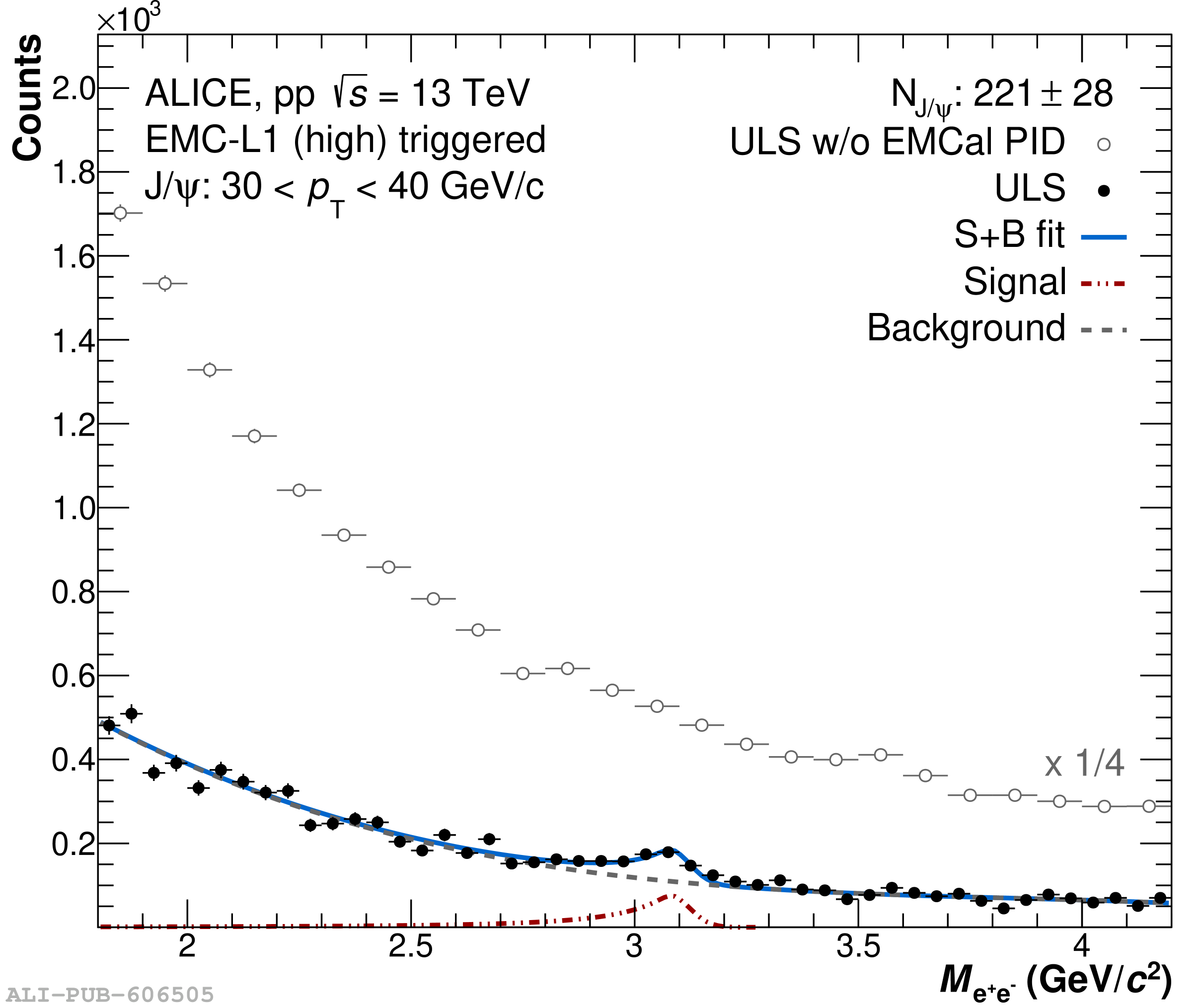 |
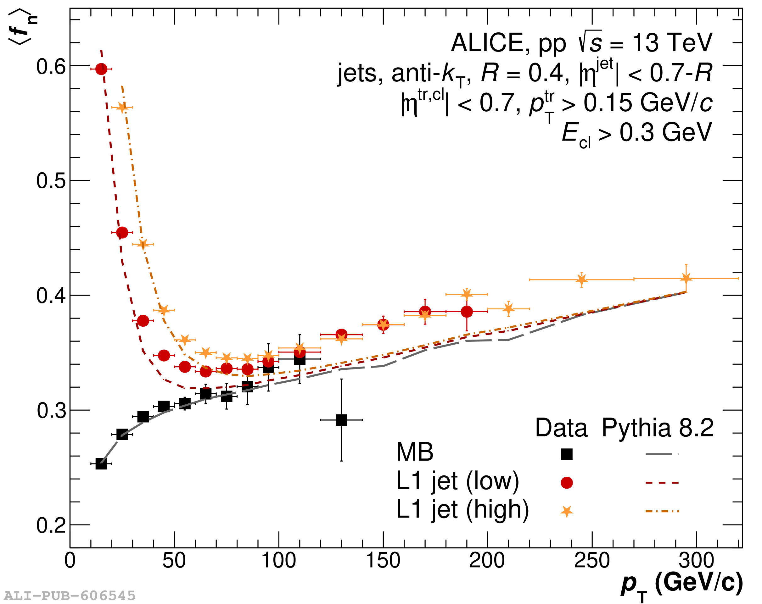
Figure 96
Instrumental effects on the jet energy measurement at $\sqrt{s}=$ 13 TeV in pp collisions as a function of the jet resolution parameter ($R=0.2$, $R=0.4$ and $R=0.6$). Upper panel: jet-by-jet distribution for various intervals in jet $p_{\rm T}$. Lower panels: JES as mean (left) and JER as standard deviation (right) of these distributions with ($f=1$) and without ($f=0$) the hadronic correction ($c_{\rm had}$), shown as points and lines, respectively. The gray bands indicate the $p_{\rm T}$ regions not taken into account for the final measurements. | 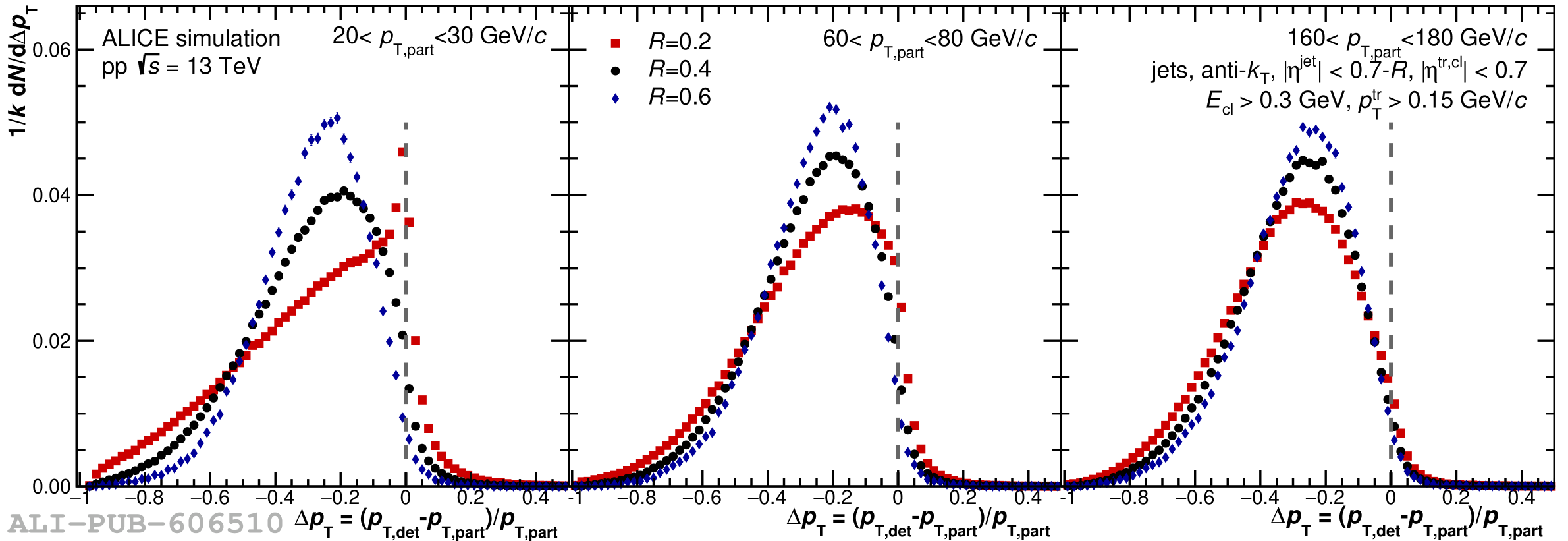 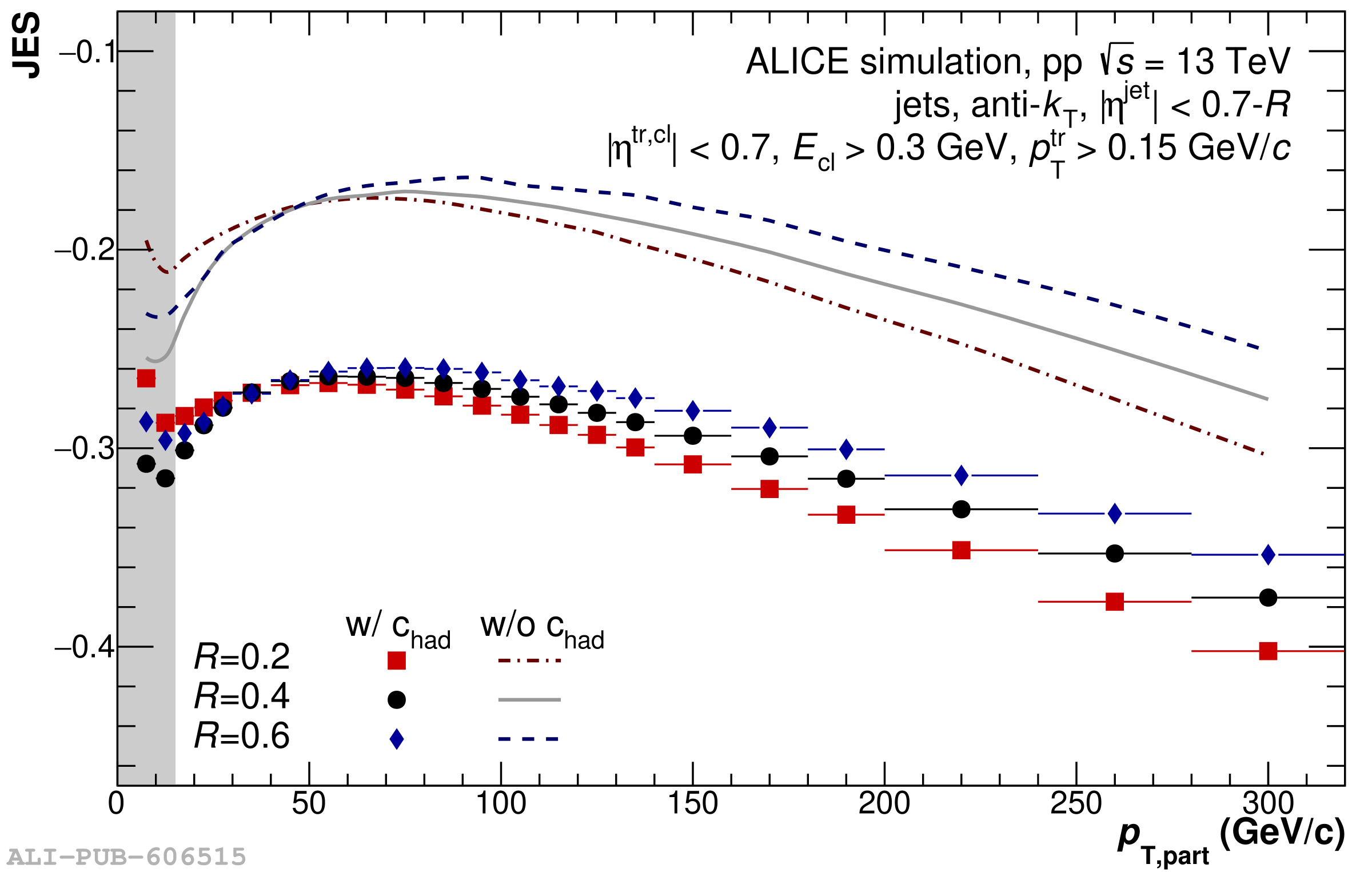 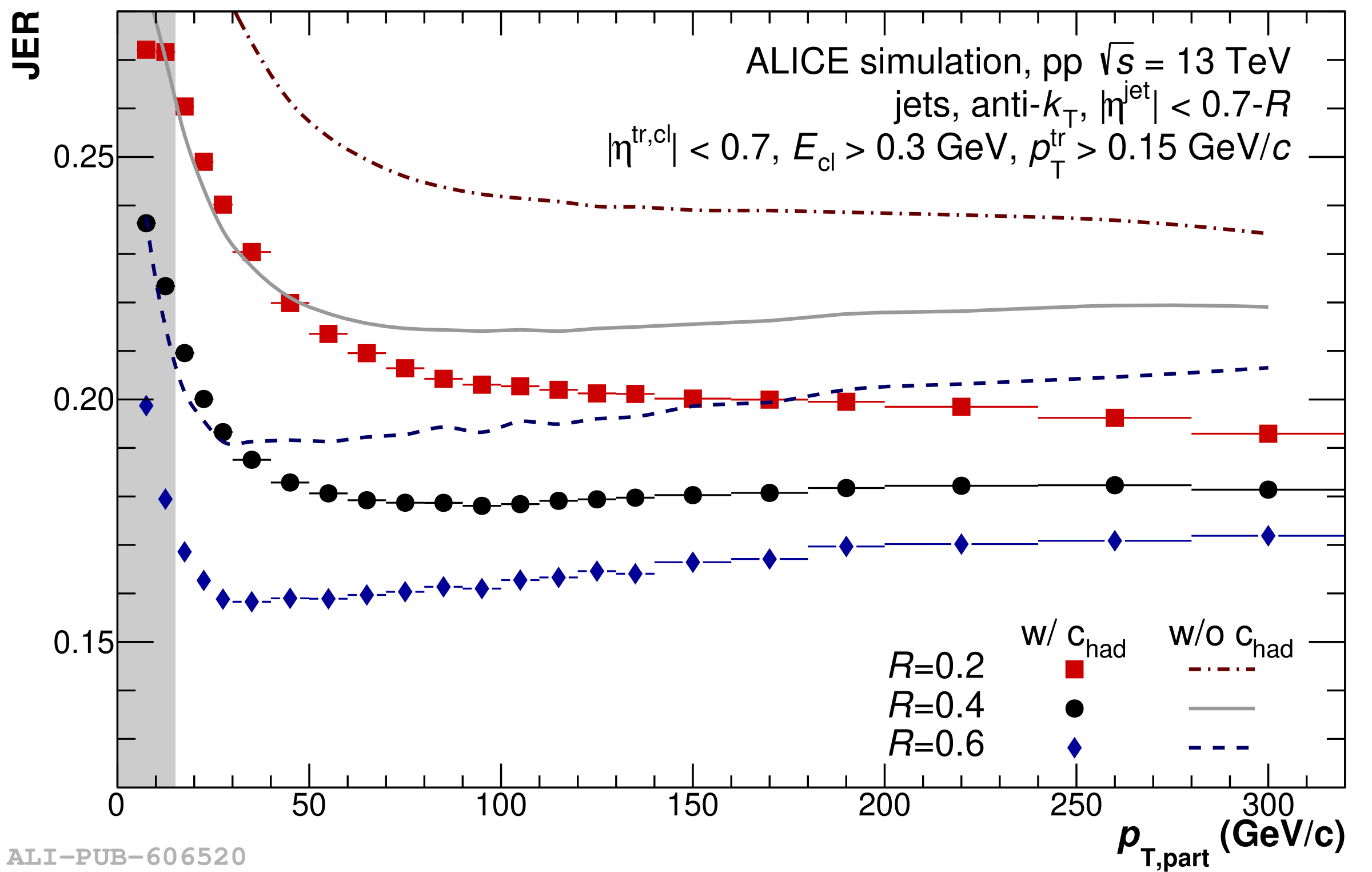 |
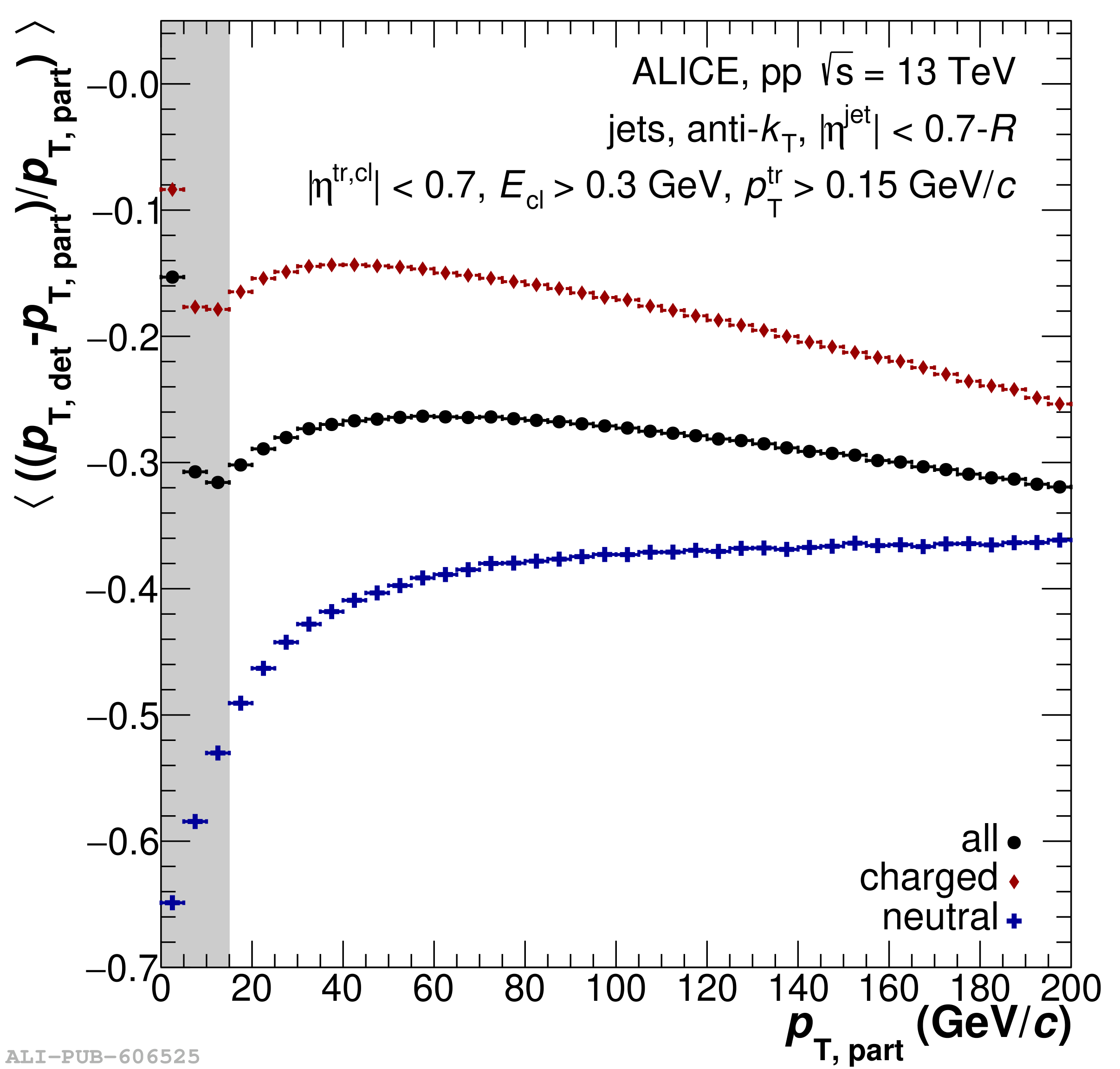
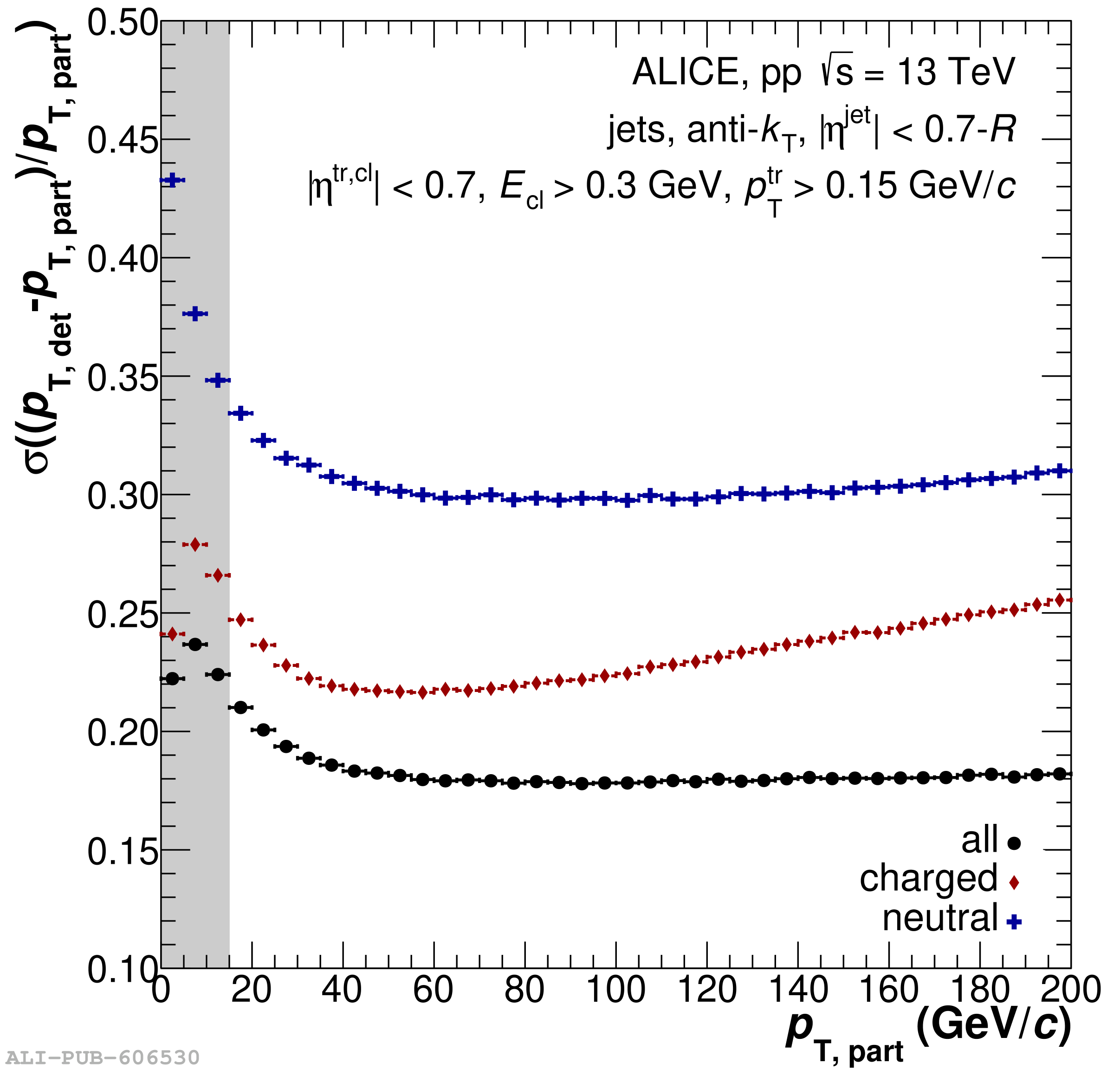
Figure 98
Jet finding efficiency $\varepsilon_{\rm jet}$ (left) and purity $P_{\rm jet}$ (right) for jets with different jet resolution parameter measured in pp collisions at $\sqrt{s}=$ 13 TeV. The gray bands indicate the $p_{\rm T}$ regions not taken into account for the final measurements. | 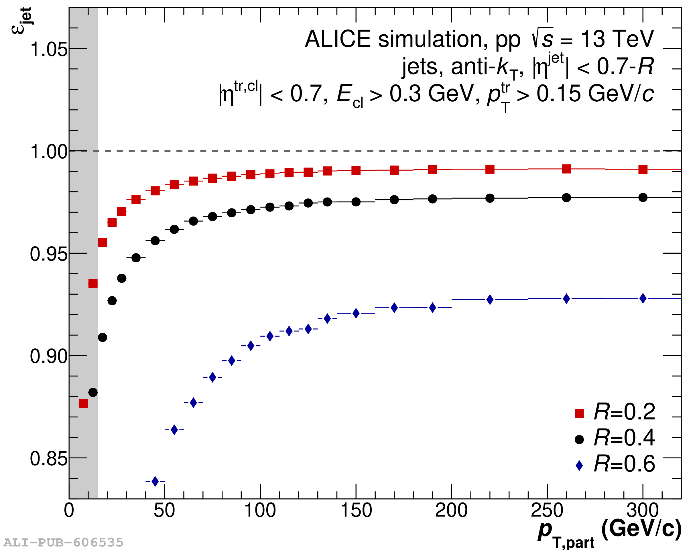 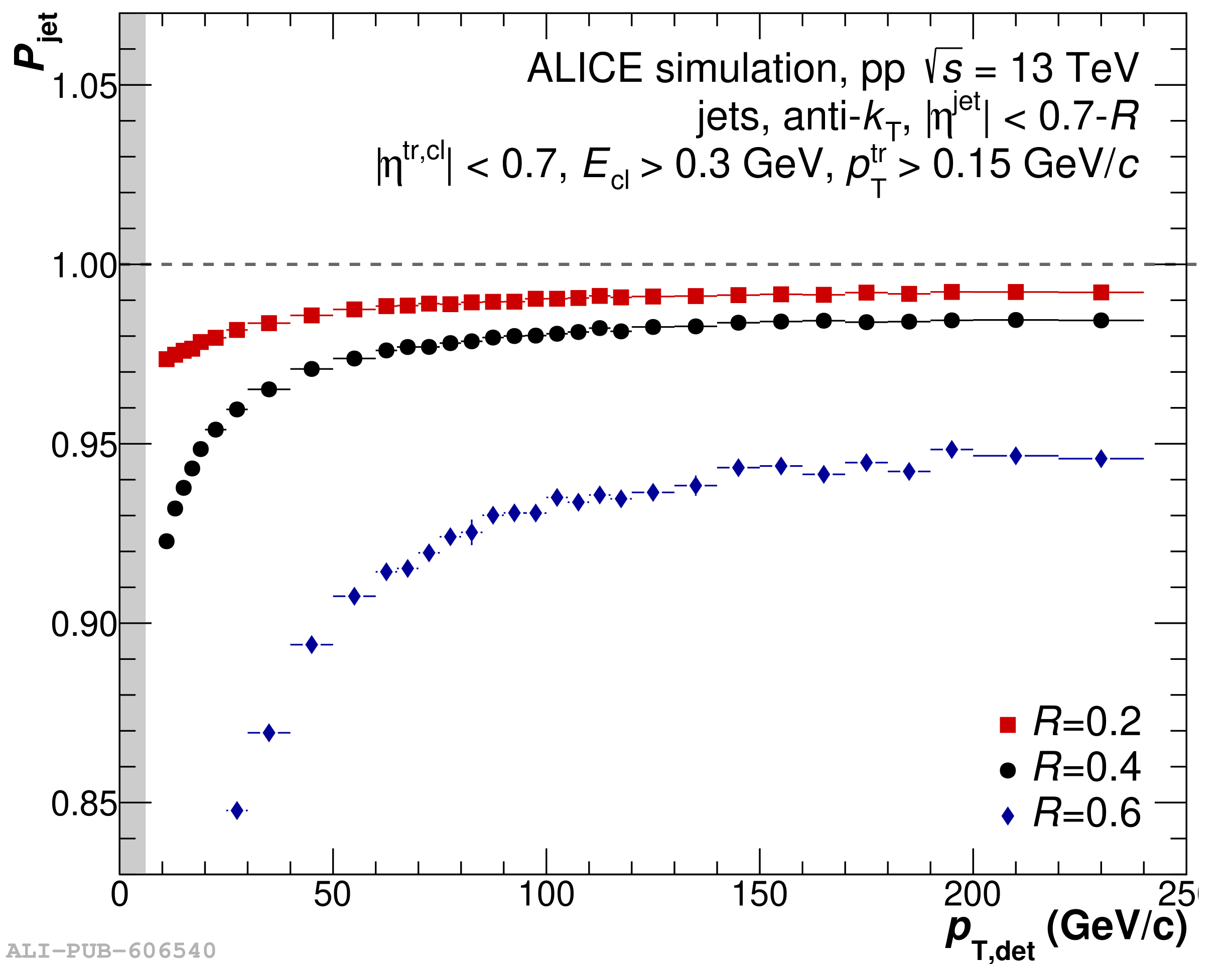 |
![[png]](https://alice-publications.web.cern.ch/sites/default/files/papers/8398/Translations.png)
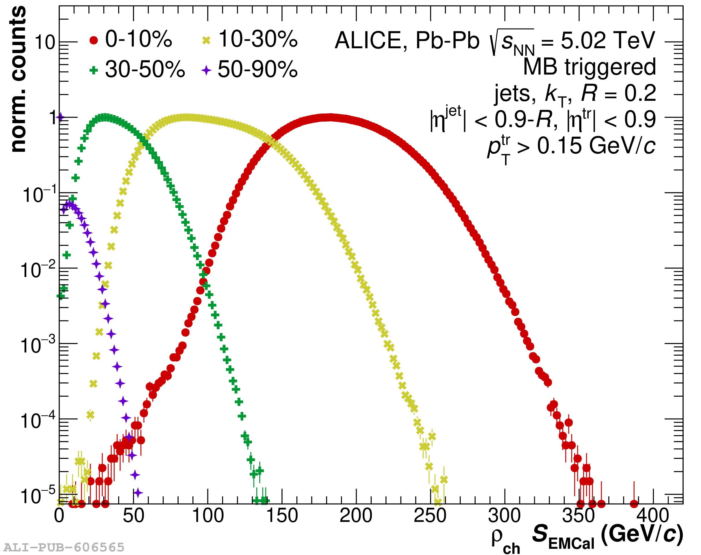
Figure 102
Left: Probability distribution of the $\delta p_{\rm T}$ distribution for random cones with radii of $R = 0.2$ and $R = 0.4$ excluding the 2 leading jets in the EMCal for the 10% most central Pb$-$Pb collisions at $\sqrt{s_{\rm NN}}=$ 5.02 TeV. On top of the distributions, the corresponding Gaussian fits for $\delta p_{\rm T}< 0$ are displayed as dashed and dotted lines Right: Comparison of the Gaussian width of the $\delta p_{\rm T}$ distribution as a function of centrality for $R = 0.2$ and $R = 0.4$ in Pb$-$Pb collisions at $\sqrt{s_{\rm NN}}=$ 5.02 TeV. | 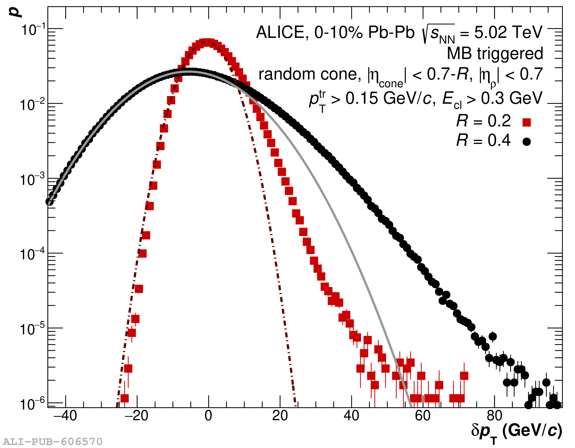  |
Figure 103
Instrumental effects on the jet energy measurement in the 0$-$10% (red) and 30$-$50% (green) central Pb$-$Pb collisions at $\sqrt{s_{\rm NN}}=5.02$ TeV for the jet resolution parameter $R=0.4$ for jets corrected with the area-based method as well as the ML-based background description for the 10% most central events (red open circle). When using the area-based correction method the jet reconstruction is done with a leading track bias of $p_{\rm T}=$ 7 GeV/$c$, while this is not the case for the machine learning based background description. For comparison, also the pp results at $\sqrt{s}=$ 5.02 TeV are shown with a leading track bias of $p_{\rm T}=$ 7 GeV/$c$ are shown in black. Upper panel: jet-by-jet distribution for various intervals in jet $p_{\rm T}$. Lower panels: the JES is the mean (left) and JER is the standard deviation (right) of these distributions. The gray bands indicate the $p_{\rm T}$ regions not taken into account for the final measurements. | 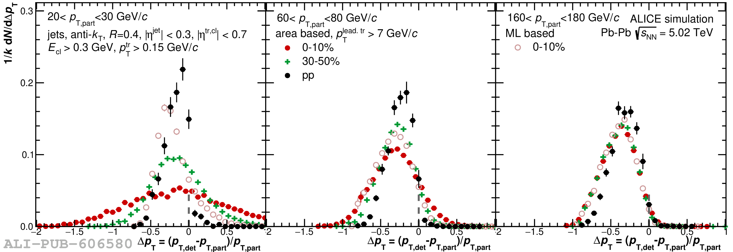 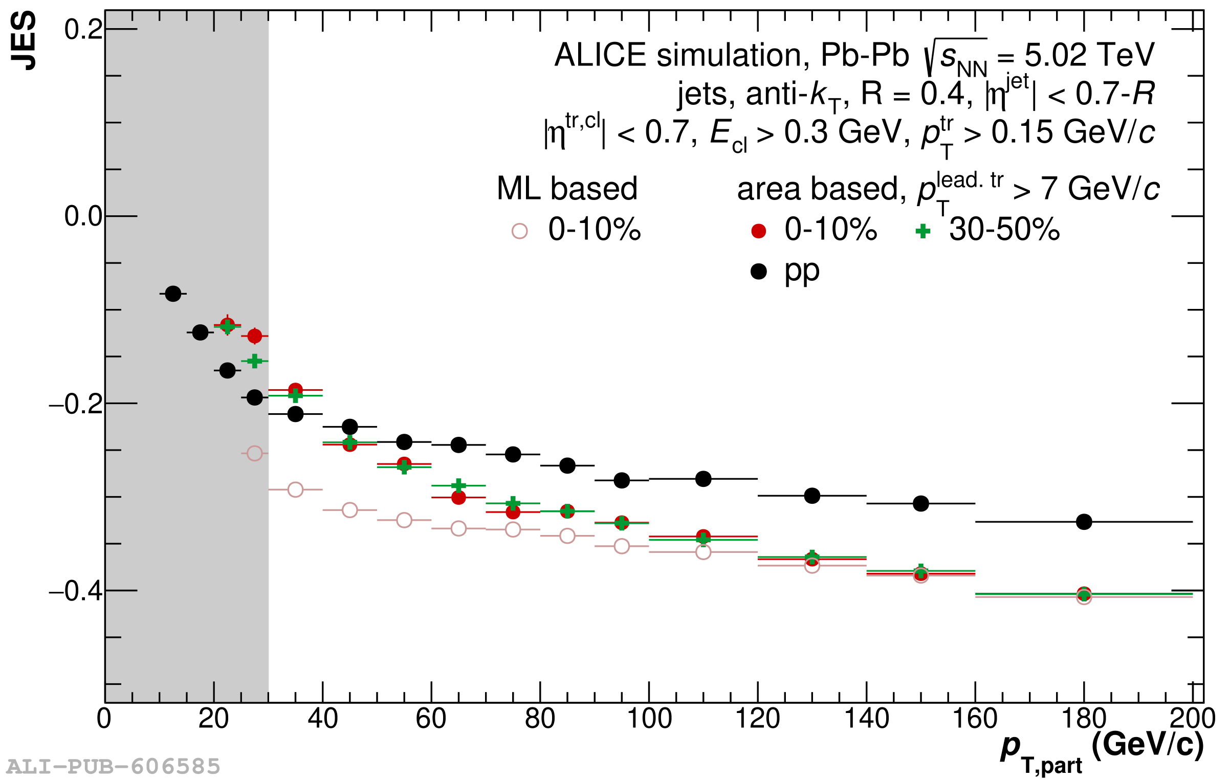 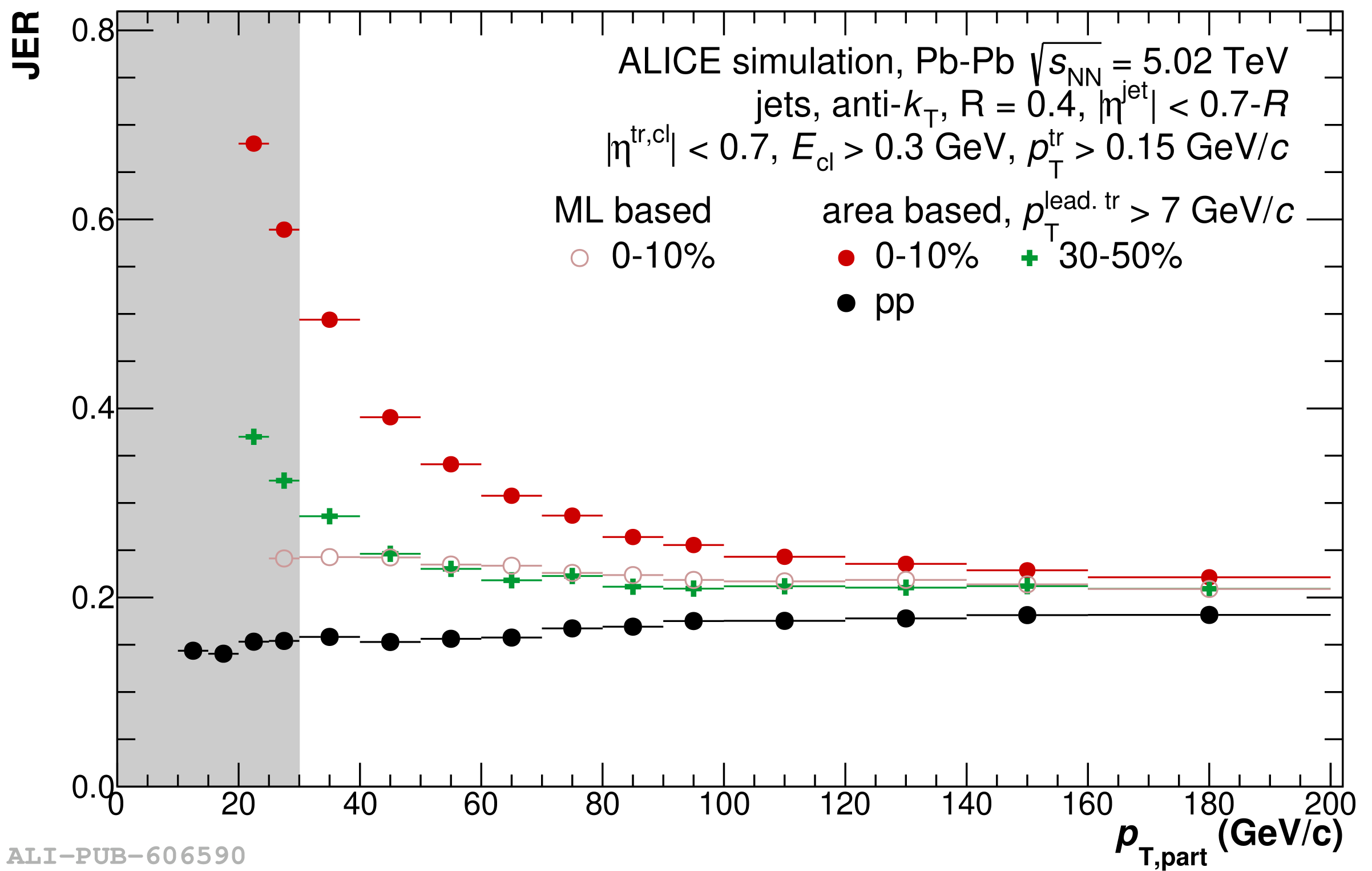 |
Figure 104
Top: Probability distribution of the $R_{g}$ residuals for jets with 60 $< p_{\rm T}< $ 80 GeV/$c$ for a jet resolution parameter of $R=0.4$ (left) and $R=0.6$ (right). Bottom: Mean (left) and width (right) of the $\Delta R_{\rm g}$ distribution versus $R_{\rm g}$ for jets with $R=0.4$ for different bins in $p_{\rm T}$. Lines denote the case where subjets were reclustered with charged constituents only. | 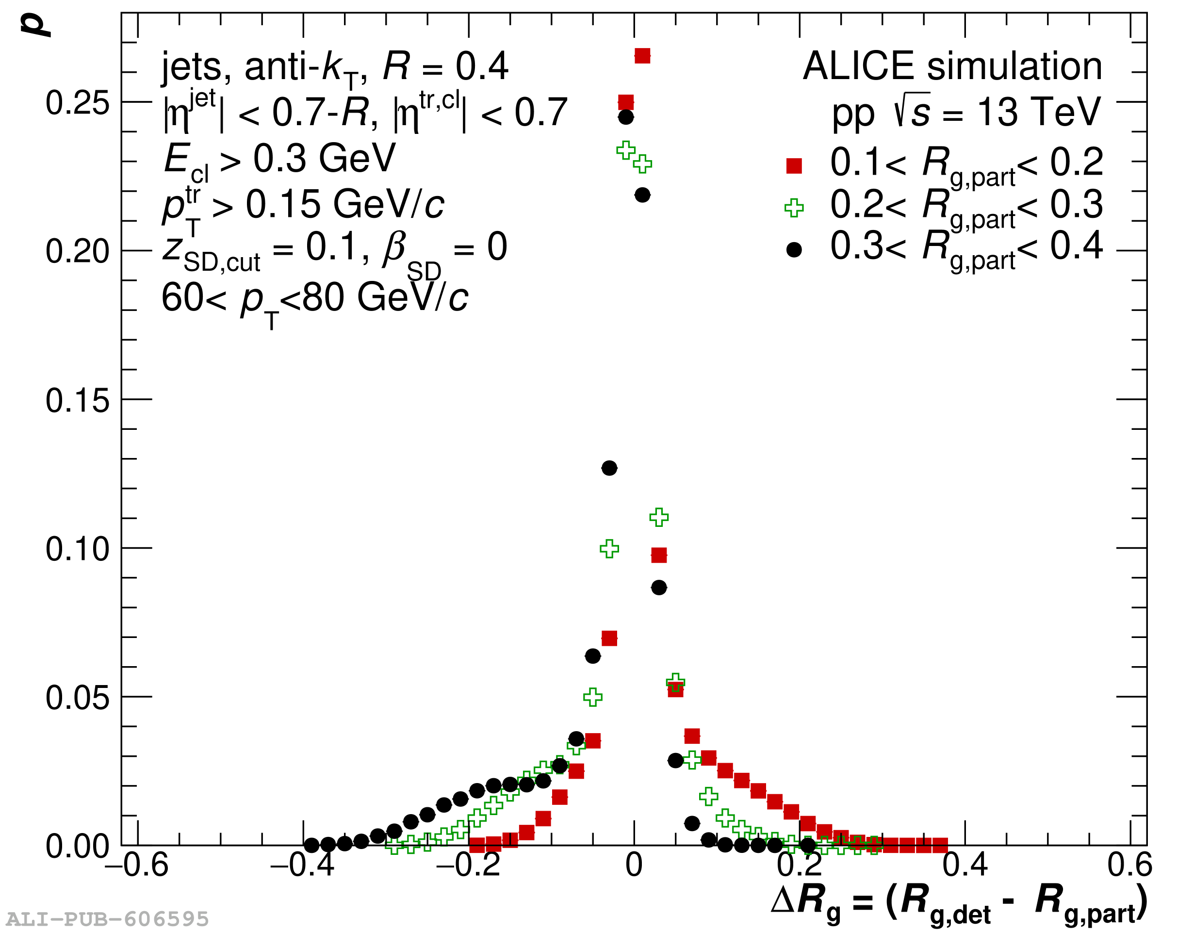 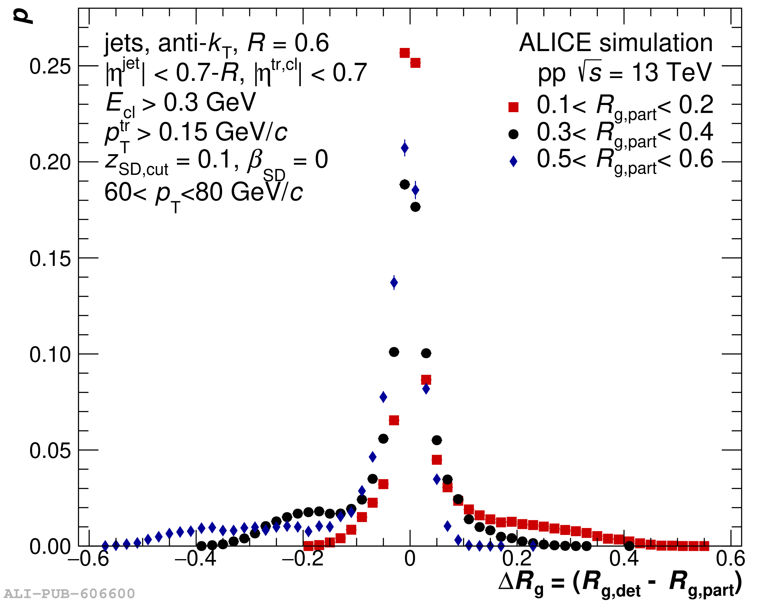  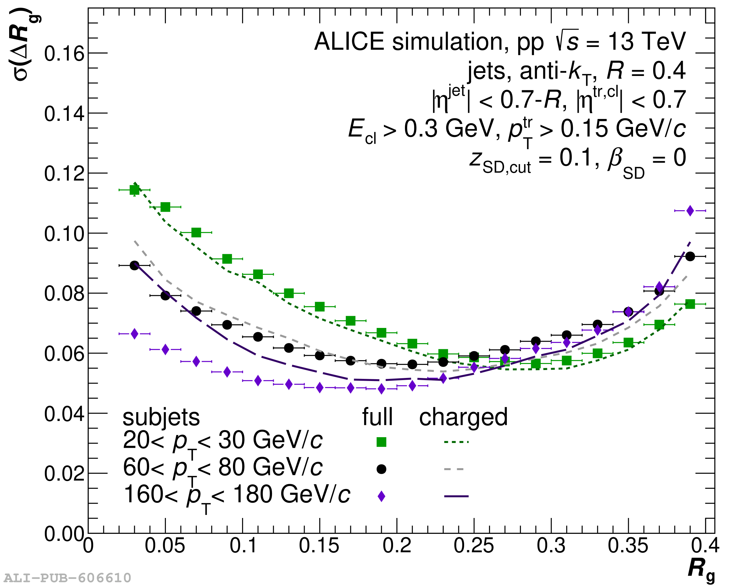 |