The measurement of primary $\pi^{\pm}$, K$^{\pm}$, p and $\overline{p}$ production at mid-rapidity ($|y| < $ 0.5) in proton-proton collisions at $\sqrt{s} = 7$ TeV performed with ALICE (A Large Ion Collider Experiment) at the Large Hadron Collider (LHC) is reported. Particle identification is performed using the specific ionization energy loss and time-of-flight information, the ring-imaging Cherenkov technique and the kink-topology identification of weak decays of charged kaons. Transverse momentum spectra are measured from 0.1 up to 3 GeV/$c$ for pions, from 0.2 up to 6 GeV/$c$ for kaons and from 0.3 up to 6 GeV/$c$ for protons. The measured spectra and particle ratios are compared with QCD-inspired models, tuned to reproduce also the earlier measurements performed at the LHC. Furthermore, the integrated particle yields and ratios as well as the average transverse momenta are compared with results at lower collision energies.
EPJC 75 (2015) 226
HEP Data
e-Print: arXiv:1504.00024 | PDF | inSPIRE
CERN-PH-EP-2015-068
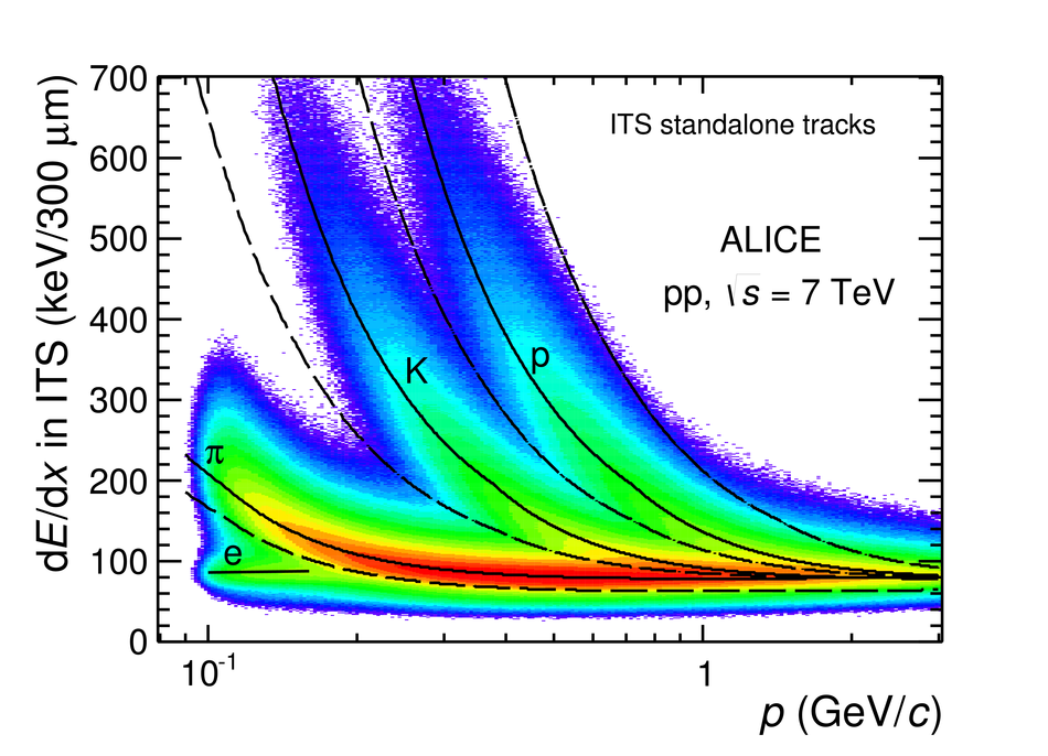
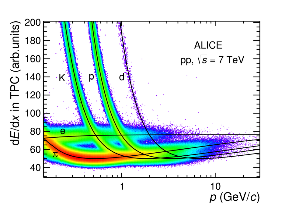
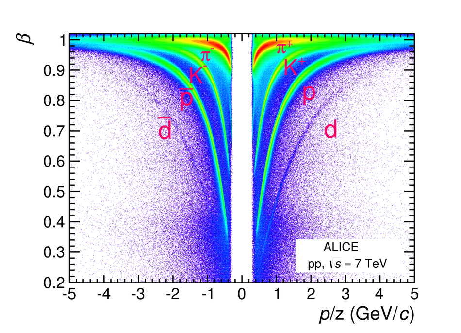
Figure 4
Distribution of $\Delta t_{i}$ assuming the pion mass hypothesis in the transverse momentum interval 1.9 $< $ $p_{\rm{T}}$ $< $ 2.0 GeV/$c$. The data (black points) are fitted with a function (light blue line) that is the sum of the signal due to pions (green dotted line) and the two populations corresponding to kaons (red dotted line) and protons (purple dashed line). | 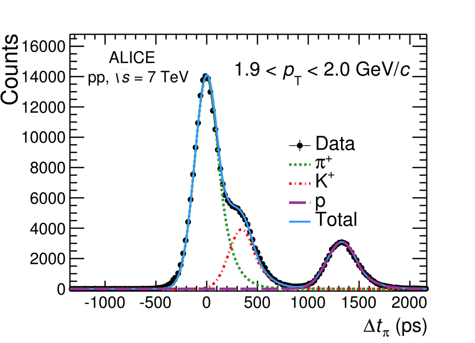 |
Figure 7
Distributions of $\langle\theta_{\rm{ckov}}\rangle$ measured with the HMPID in the two narrow $p_{\rm{T}}$ intervals 3.4 < $p_{\rm{T}}$ $< $ 3.6 GeV/$c$ (top) and 5 < $p_{\rm{T}}$ < 5.5 GeV/$c$ (bottom) for tracks from negatively-charged particles. Solid lines represent the total fit (sum of three Gaussian functions). Dotted lines correspond to pion, kaon and proton signals. The background is negligible. | 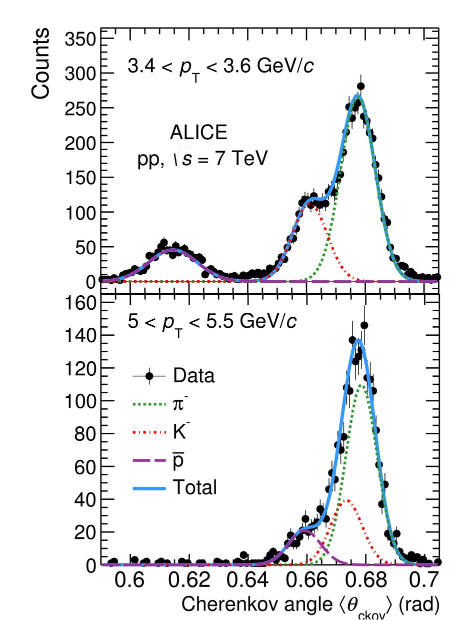 |
Figure 8
Separation power ($n_{\sigma}$) of hadron identification in the HMPID as a function of $p_{\rm{T}}$. The separation n$_{\sigma}$ of pions and kaons (kaons and protons) is defined as the difference between the average of the Gaussian distributions of $\langle\theta_{\rm{ckov}}\rangle$ for the two hadron species divided by the average of the Gaussian widths of the two distributions. |  |
Figure 9
Kink invariant mass $M_{\mu\nu}$ in data (red circles) and Monte-Carlo (black line) for summed particles and antiparticles, integrated over the mother transverse momentum range 0.2 < $p_{\rm{T}}$ < 6.0 GeV/$c$ and $|y| < 0.7$ before (top panel) and after (bottom panel) the topological selections, based mainly on the $q_\mathrm{T}$ and the maximum decay opening angle. | 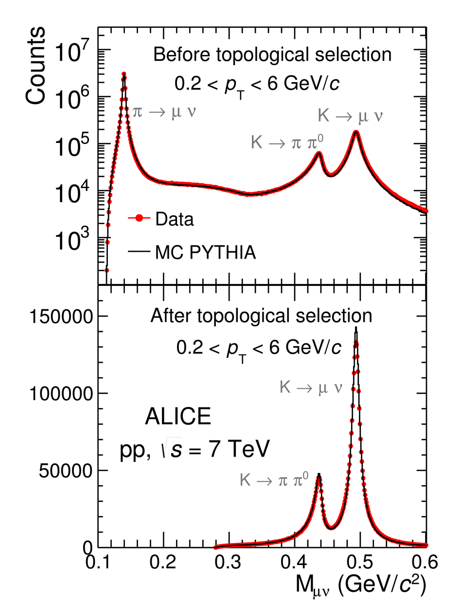 |
Figure 10
Proton DCA$_{xy}$ distribution in the range 0.55 < $p_{\rm{T}}$< 0.60GeV/$c$ together with the Monte-Carlo templates for primary protons (green dotted line), secondary protons from weak decays (red dotted line) and secondary protons produced in interactions with the detector material (blue dashed line) which are fitted to the data. The light blue line represents the combined fit, while the black dots are the data. | 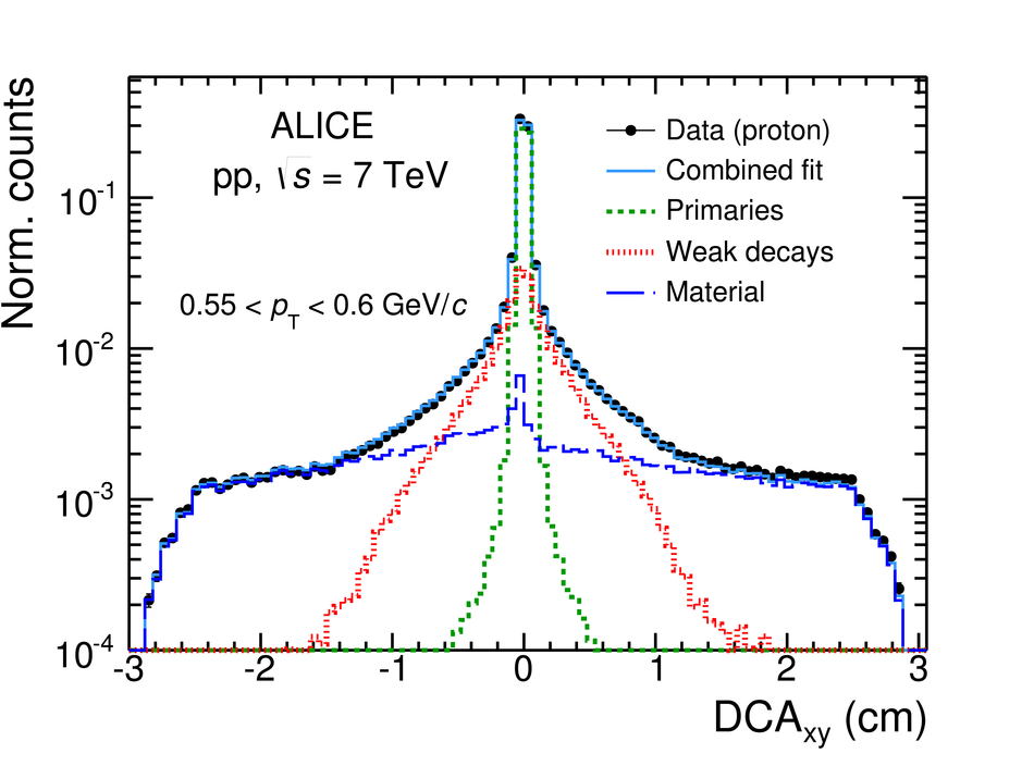 |
Figure 11
Correction factors ($\varepsilon$($p_{\rm{T}}$) in Eq. 2) for $\pi^{+}$, K$^{+}$ and p (left panel) and their antiparticles (right panel) accounting for PID efficiency, detector acceptance, reconstruction and selection efficiencies for ITS-sa (red circles), TPC-TOF (light blue squares), TOF (green diamonds), HMPID (black stars) and kink (purple crosses) analyses. | 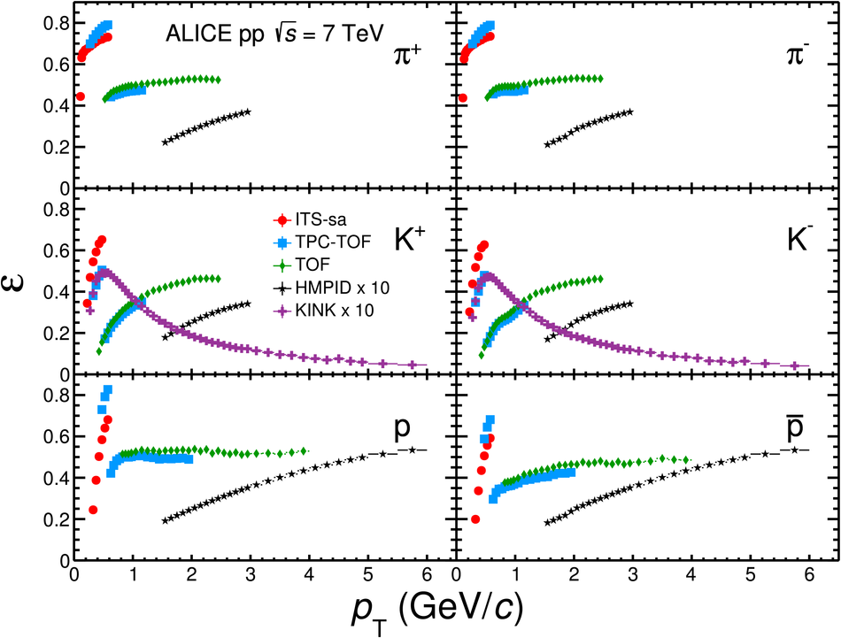 |
Figure 12
Top panel: $p_{\rm{T}}$ spectra of $\pi$, K and p, sum of particles and antiparticles, measured with ALICE at mid-rapidity ($|y| < $ 0.5) in pp collisions at $\sqrt{s}=$ 7 TeV by using different PID techniques. The spectra are normalized to the number of inelastic collisions. Statistical (vertical error bars) and systematic (open boxes) uncertainties are reported. The horizontal width of the boxes represents the $p_{\rm{T}}$-bin width The markers are placed at the bin centre Bottom panels: ratio between the spectra obtained from each analysis and the combined one. The error bands represent the total systematic uncertainties for each analysis. The uncertainty due to the normalization to inelastic collisions ($ ^{+7}_{-4} \%$), common to the five PID analyses, is not included. | 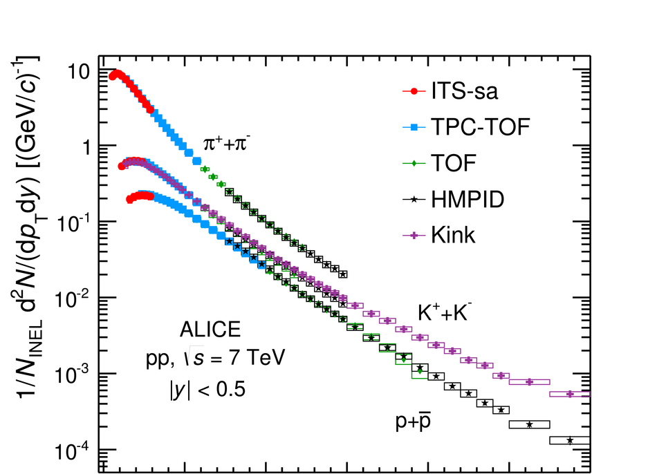 |
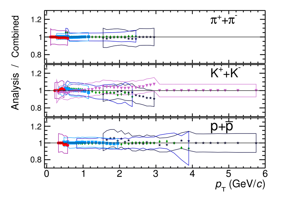
Figure 13
Combined $p_{\rm{T}}$ spectra of $\pi$, K and p, sum of particles and antiparticles, measured with ALICE at mid-rapidity ($|y| < $ 0.5) in pp collisions at $\sqrt{s}=$ 7 TeV normalized to the number of inelastic collisions. Statistical (vertical error bars) and systematic (open boxes) uncertainties are reported. The uncertainty due to the normalization to inelastic collisions ($ ^{+7}_{-4} \%$) is not shown. The spectra are fitted with Lévy-Tsallis functions. |  |
Figure 14
Comparison of $p_{\rm{T}}$ spectra of $\pi$, K and p (sum of particles and antiparticles) measured by the ALICE ($|y|< 0.5$) and CMS Collaborations ($|y|< 1$) in pp collisions at $\sqrt{s}$ = 7 TeV. The CMS data points are scaled by the empirical factor 0.78, as described in . Inset plot: Ratios between ALICE and CMS data in the common $p_{\rm{T}}$ range. The combined ALICE and CMS statistical (vertical error bars) and systematic (open boxes) uncertainties are reported. The combined ALICE ($ ^{+7}_{-4} \%$) and CMS ($\pm 3\%$) normalization uncertainty is shown as a grey box around 1 and not included in the point-to-point uncertainties. | 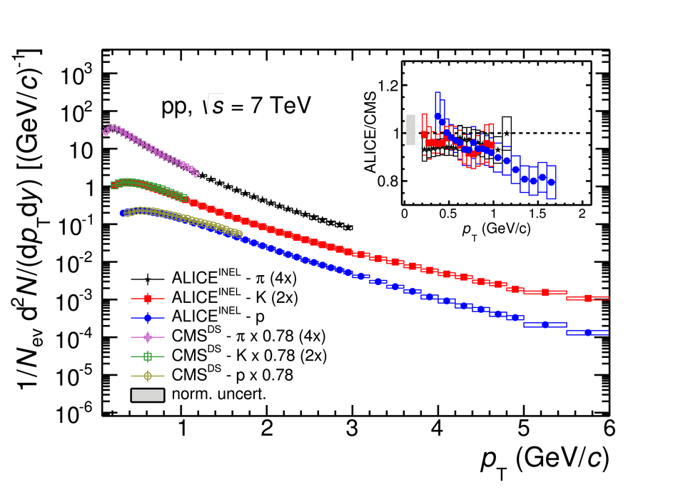 |
Figure 15
$p_{\rm{T}}$-integrated yields d$N/$d$y$ of $\pi$, K and p as a function of the centre-of-mass energy in pp collisions. PHENIX results are for separate charges while CMS and ALICE results are the average of the d$N/$d$y$ of particles and antiparticles. ALICE and CMS points are slightly shifted along the x-axis for a better visualization. Errors (open boxes) are the combination of statistical (negligible), systematic and normalization uncertainties. | 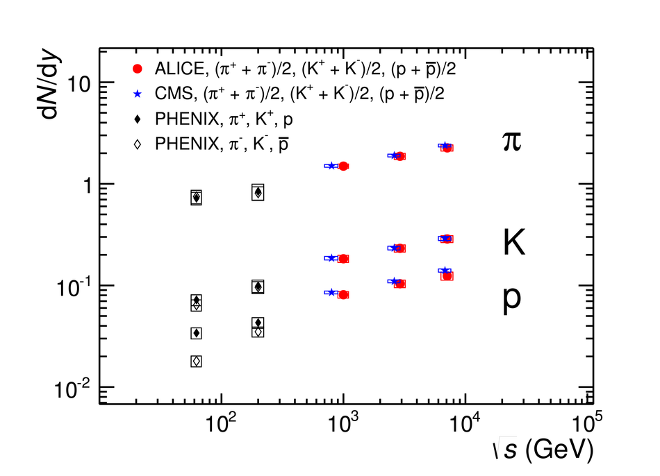 |
Figure 16
(K$^{+}$+K$^{-}$)/($\pi^{+}$+$\pi^{-}$) (top) and (p+$\rm\overline{p}$)/($\pi^{+}$+$\pi^{-}$) (bottom) ratios in pp and p$\overline{\mathrm{p}}$ collisions as a function of the collision energy $\sqrt{s}$ Errors (open boxes) are the combination of statistical (negligible) and systematic uncertainties. | 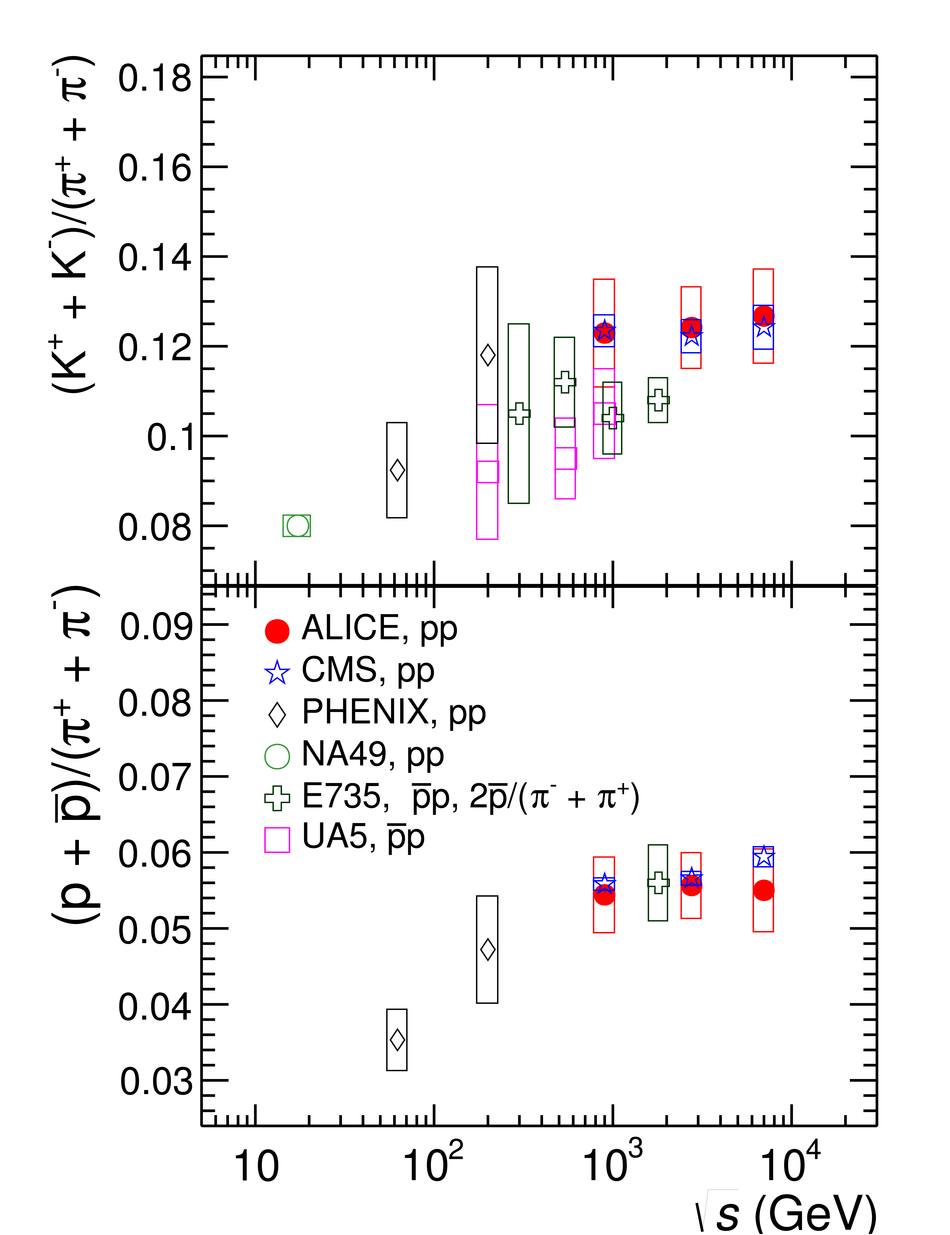 |

Figure 18
Top panel: Measured $p_{\rm{T}}$ spectra of pions, kaons and protons, sum of particles and antiparticles, compared to PYTHIA6-Z2, PYTHIA6-CentralPerugia2011, PYTHIA8, EPOS LHC and PHOJET Monte-Carlo calculations. Statistical (vertical error bars) and systematic (open boxes) uncertainties are reported for the measured spectra. Bottom panels: ratios between data and Monte-Carlo calculations. | 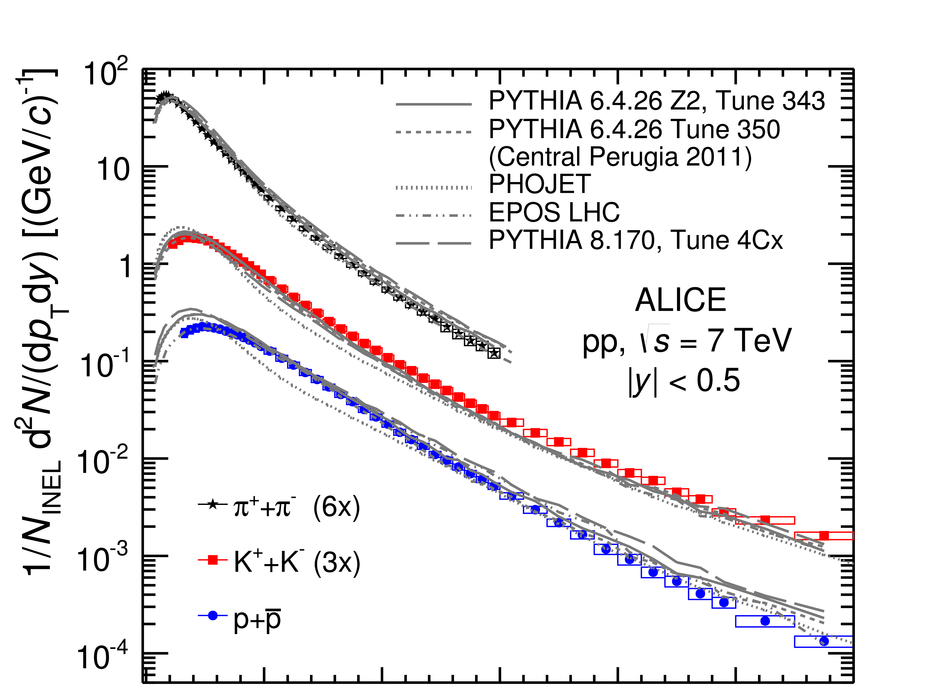 |
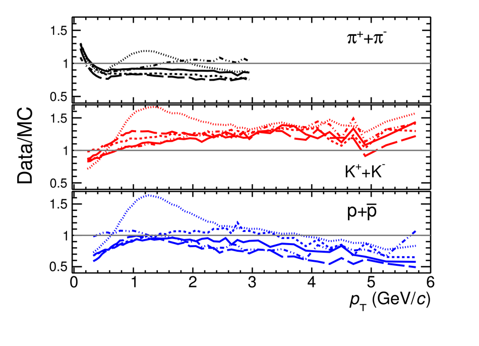
Figure 19
Measured (K$^{+}$+K$^{-}$)/($\pi^{+}$+$\pi^{-})$ (left) and (p+$\rm\overline{p}$)/($\pi^{+}$+$\pi^{-})$ (right) ratios as a function of $p_{\rm{T}}$ compared to PYTHIA6-Z2, PYTHIA6-CentralPerugia2011, PYTHIA8, EPOS LHC and PHOJET calculations. Statistical (vertical error bars) and systematic (open boxes) uncertainties are reported for the measured spectra. | 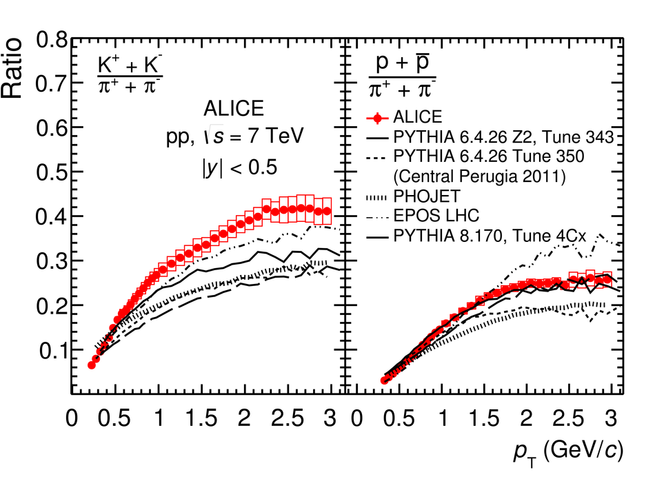 |