In our Galaxy, light antinuclei composed of antiprotons and antineutrons can be produced through high-energy cosmic-ray collisions with the interstellar medium or could also originate from the annihilation of dark-matter particles that have not yet been discovered. On Earth, the only way to produce and study antinuclei with high precision is to create them at high-energy particle accelerators. Although the properties of elementary antiparticles have been studied in detail, the knowledge of the interaction of light antinuclei with matter is limited. We determine the disappearance probability of $^{3}\overline{\rm He}$ when it encounters matter particles and annihilates or disintegrates within the ALICE detector at the Large Hadron Collider. We extract the inelastic interaction cross section, which is then used as input to calculations of the transparency of our Galaxy to the propagation of $^{3}\overline{\rm He}$ stemming from dark-matter annihilation and cosmic-ray interactions within the interstellar medium. For a specific dark-matter profile, we estimate a transparency of about 50%, whereas it varies with increasing $^{3}\overline{\rm He}$ momentum from 25% to 90% for cosmic-ray sources. The results indicate that $^{3}\overline{\rm He}$ nuclei can travel long distances in the Galaxy, and can be used to study cosmic-ray interactions and dark-matter annihilation.
Nature Physics volume 19, pages 61–71 (2023)
HEP Data
e-Print: arXiv:2202.01549 | PDF | inSPIRE
CERN-EP-2022-023
Figure group
Figure 1
Description of the steps followed for the extraction of \sigmainel. (a) Schematic of the ALICE detectors at midrapidity in the plane perpendicular to the beam axis, with the collision point located in the middle; the ITS, TPC, TRD and TOF detectors are shown in green, blue, yellow and orange, respectively. A \ahe\ which annihilates in the TPC gas is shown in red, and a \he\ that does not undergo an inelastic reaction and reaches the TOF detector in blue; the dashed curves represent charged (anti)particles produced in the \ahe\ annihilation. (b) Identification of (anti)nuclei by means of their specific energy loss d$E$/d$x$ and momentum measurement in the TPC. The red points show all (anti)$^{3}$He nuclei reconstructed with the TPC detector, blue points correspond to (anti)$^{3}$He with TOF information; other (anti)particles are shown in black. (c) Experimental results for the raw ratio of \ahe\ to \he\ in pp collisions at $\sqrt{s} = 13$ TeV as a function of rigidity. The vertical lines and boxes represent statistical and systematic uncertainties in terms of standard deviations, respectively. The black and red lines show the results from the Monte Carlo simulations with varied \sigmainel. (d) Experimental ratio of \ahe\ with TOF information over \ahe\ reconstructed in the TPC in the 10\% most central Pb--Pb collisions at $\sqrt{s_{\rm NN}} = 5.02$ TeV as a function of rigidity. The black and red lines show the results from the Monte Carlo simulations with varied \sigmainel. (e) The raw ratio of \ahe\ to \he\ in a particular rigidity interval as a function of \sigmainel\ for $\langle A\rangle = 17.4$. The fit to the results from Monte Carlo simulations (black points) shows the dependence of the observable on \sigmainel\ according to the Lambert--Beer formula. The horizontal dashed blue lines show the central value and $1\sigma$ uncertainties for the measured observable and their intersection with the Lambert--Beer function determines \sigmainel\ limits (yellow lines). (f) Extraction of \sigmainel\ for $\langle A\rangle = 34.7$ analogous to the panel e, with \sigmainel\ limits shown as magenta lines. | 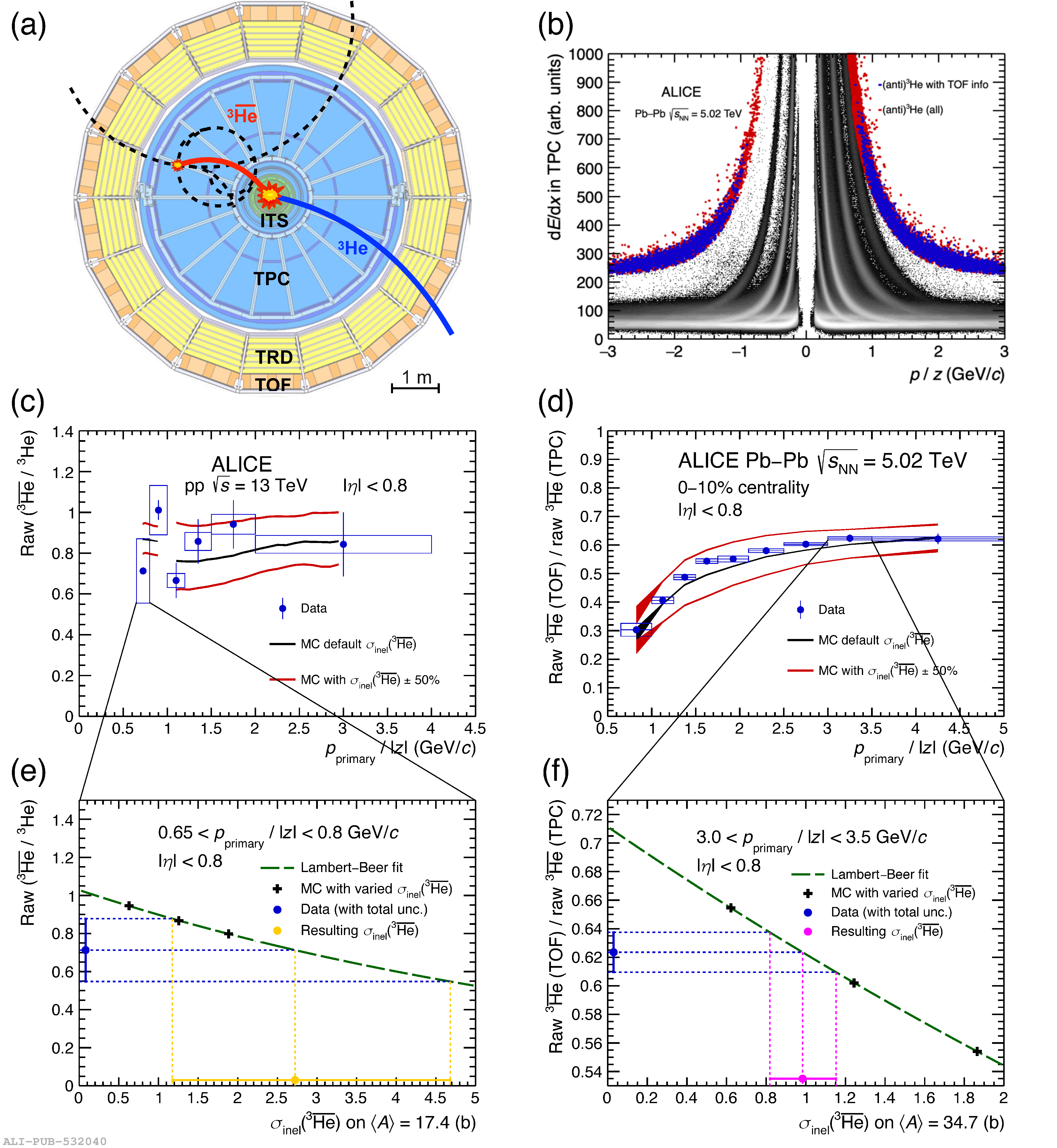 |
Figure 2
Results for \sigmainel\ as a function of \ahe\ momentum. Results obtained from pp collisions at $\sqrt{s} =$ 13 TeV (left); results from the 10\% most central Pb--Pb collisions at $\sqrt{s_{\mathrm{NN}}} =\, 5.02$ TeV (right). The curves represent the \geant cross sections corresponding to the effective material probed by the different analyses. The arrow on the left plot shows the 95\% confidence limit on \sigmainel\ for $\langle A \rangle =$ 17.4. The different values of $\langle A \rangle$ correspond to the three different effective targets (see the main text for details). All the indicated uncertainties represent standard deviations. | 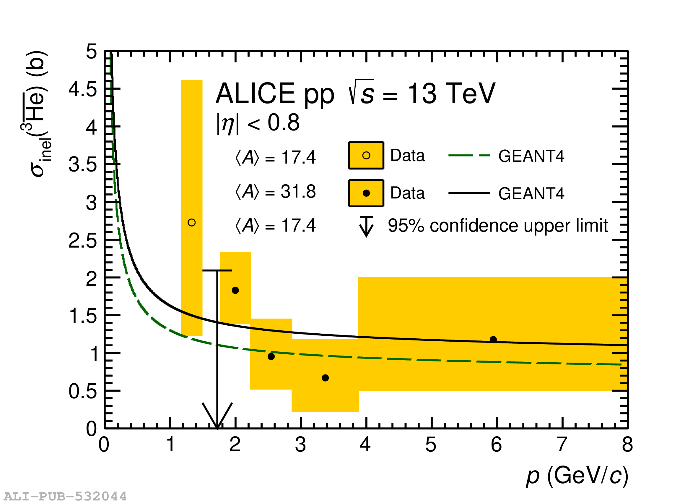 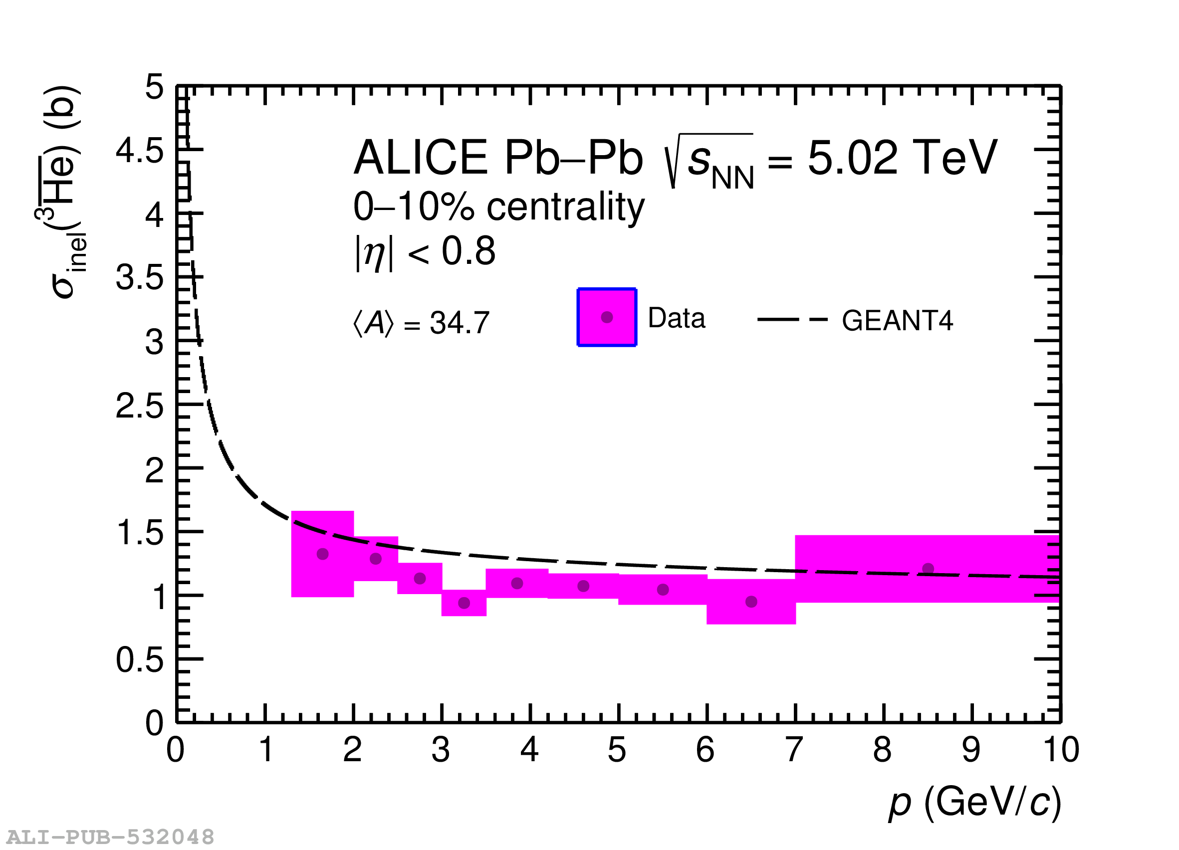 |
Figure 3
Schematic of \ahe\ production and propagation in our Galaxy. Distribution of DM density $\rho_{\rm DM}$ in our Galaxy as a function of the distance from the galactic centre according to the Navarro–Frenk–White profile (top). Graphical illustration of the \ahe\ production from cosmic-ray interactions with interstellar gas or DM ($\chi$) annihilations (bottom). The yellow halo represents the heliosphere and the Earth, Sun and positions of the Voyager 1, AMS-02 and GAPS experiments are depicted, too. |  |
Figure 4
Expected \ahe\ flux near Earth before and after solar modulation. Data before (left) and after (right) solar modulation. The latter is obtained using the force-field method with modulation potential $\mathrm{\phi} =$ 400 MV. The results are shown as a function of kinetic energy per nucleon $E_{\rm kin} / A$. Fluxes for DM signal $\chi$ (red) and cosmic-ray background (blue) antihelium nuclei for different cases of inelastic cross section used in the calculations (top). The bands show the results obtained with \sigmainel\ from ALICE measurements, and the full lines correspond to the results using the \geant\ parameterizations. The dashed lines show the fluxes obtained with \sigmainel\ set to zero for DM signal (orange line) and for cosmic-ray background (magenta line). The green band on the x axis indicates the kinetic energy range corresponding to the ALICE measurement for \sigmainel. Transparency of our Galaxy to the propagation of \ahe\ outside (left) and inside (right) the Solar System (bottom). The shaded areas (top right) show the expected sensitivity of the GAPS and AMS-02 experiments. The top panels also shows the fluxes obtained with \sigmainel\ set to zero. Only the uncertainties relative to the measured \sigmainel\ are shown, which represent standard deviations. The calculations employ the \ahe\ DM source described elsewhere and the \ahe\ production cross section from cosmic-ray background . | 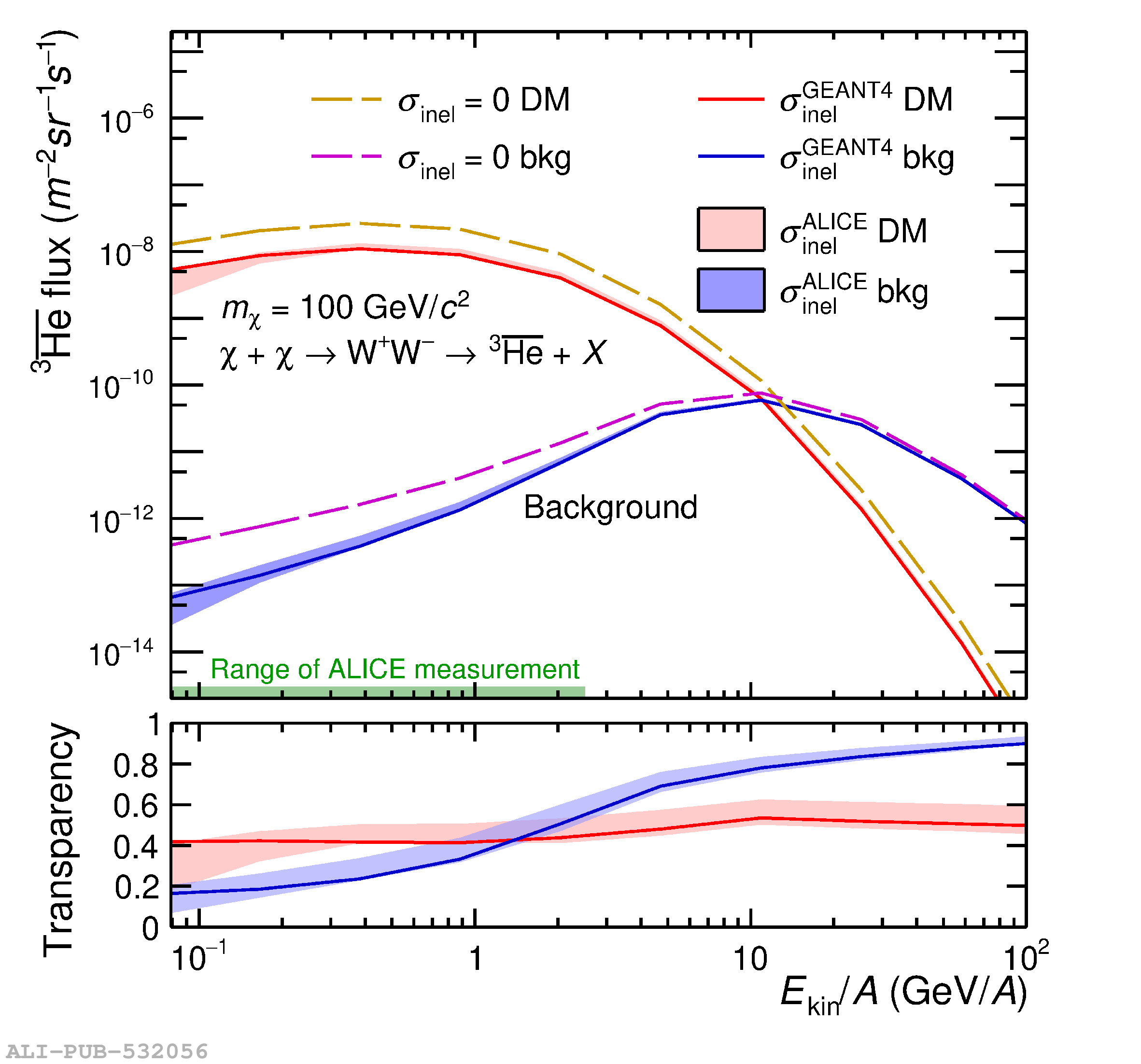  |
Figure 5
Inelastic cross section for \ahe\ on protons (left) and on $^{4}$He (right). The green band shows the scaled ALICE measurement (see text for details), the red line represents the original \geant parameterization and the black line on the left plot the parameterization employed in Ref. . The width of the green band represents standard deviation uncertainty. The blue band on the x axis indicates the kinetic energy range corresponding to the ALICE measurement for \sigmainel. | 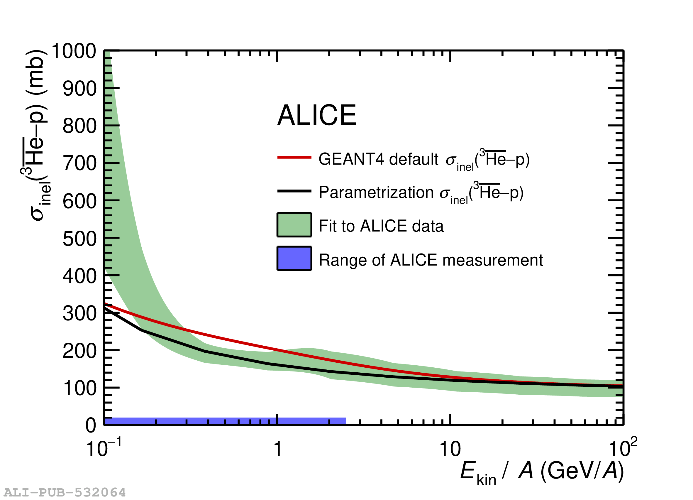  |