ALICE is the heavy-ion experiment at the CERN Large Hadron Collider. The experiment continuously took data during the first physics campaign of the machine from fall 2009 until early 2013, using proton and lead-ion beams. In this paper we describe the running environment and the data handling procedures, and discuss the performance of the ALICE detectors and analysis methods for various physics observables.
Int. J. Mod. Phys. A 29 (2014) 1430044
e-Print: arXiv:1402.4476 | PDF | inSPIRE
CERN-PH-EP-2014-031
Figure 1
The ALICE experiment at the CERN LHC. The central-barrel detectors (ITS, TPC, TRD, TOF, PHOS, EMCal, and HMPID) are embedded in a solenoid with magnetic field B=0.5 T and address particle production at midrapidity. The cosmic-ray trigger detector ACORDE is positioned on top of the magnet. Forward detectors (PMD, FMD, V0, T0, and ZDC) are used for triggering, event characterization, and multiplicity studies. The MUON spectrometer covers $-4.0< \eta< -2.5$, $\eta=-\ln\tan(\theta\!/2)$ | 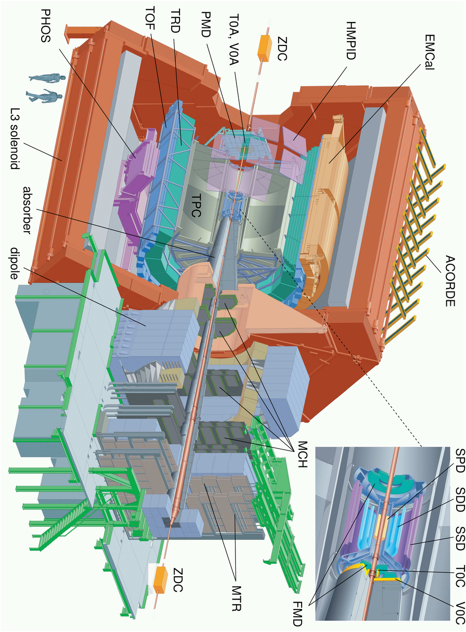 |

Figure 3
Beam pipe pressure and background rate infill 2181. The expected background rate has been estimated using the linear parameterization shown in Fig. 2. VGPB.120.4L2, VGPB.231.4L2, and VGI.514.4L2 are the pressure gauges located in front of the Inner triplet (at 69.7 m from IP2), on the TDI beam stopper (at 80 m from IP2), and on the large recombination chamber (at 109 m from IP2), respectively. | 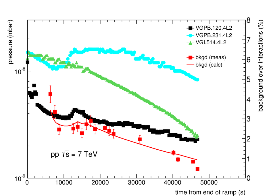 |
Figure 4
Top: minimum bias, centrality, and muon triggers as a function of time during Pb-Pb data taking (run 169721). The B mask selects the LHC bunch slots where collisions between bunches of Beam 1 and Beam 2 are expected at IP2, while the ACE mask selects slots where no beam-beam collision is expected. Bottom: ZDC-A trigger rate as a function of time in the same run. | 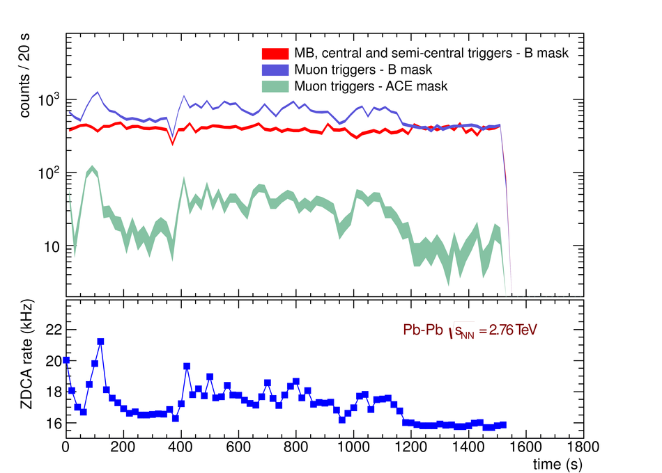 |
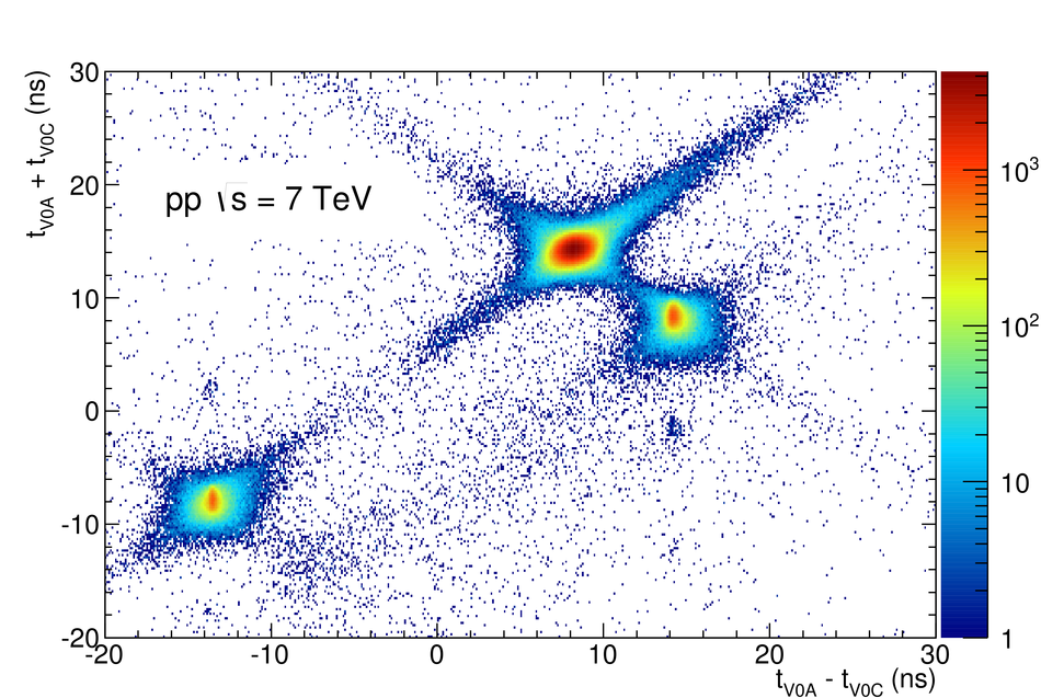
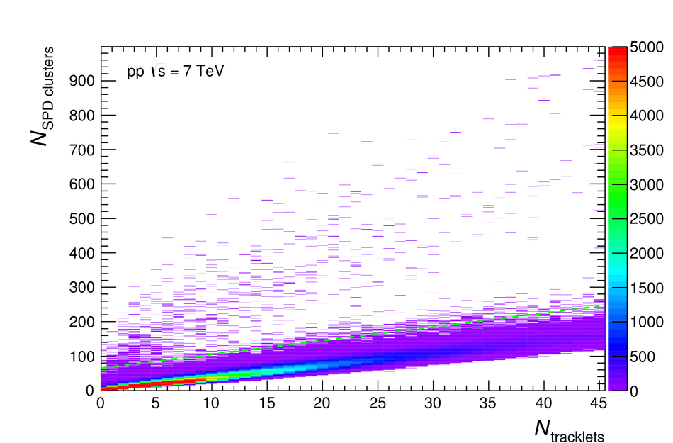
Figure 7
Correlation between the sum and the difference of times recorded by the neutron ZDCs on either side (ZNA and ZNC) in Pb-Pb collisions. The large cluster in the middle corresponds to collisions between ions in the nominal RF bucket on both sides, while the small clusters along the diagonals (spaced by 2.5 ns in the time difference) correspond to collisions in which one of the ions is displaced by one or more RF buckets. | 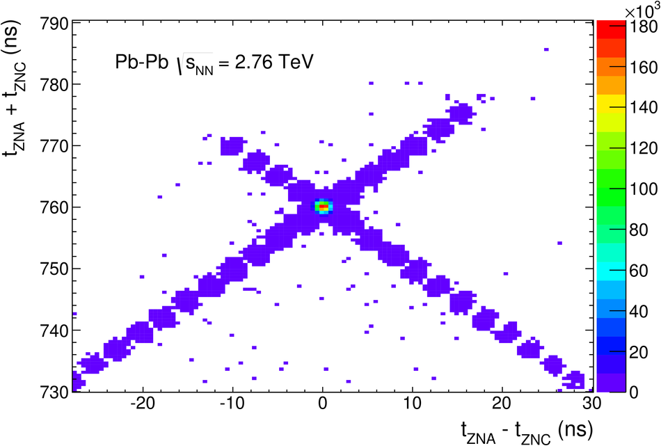 |
Figure 8
Top: MBand trigger rate vs. beam separation in $x$ and $y$ obtained during the May 2010 van der Meer scan. Double Gaussian fits to the data are shown as lines. Bottom: Measured MBand cross section for 48 colliding bunch pairs in the March 2011 scan, as a function of the product of colliding bunch intensities N$_1$N$_2$. | 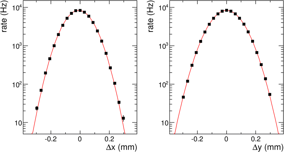 |
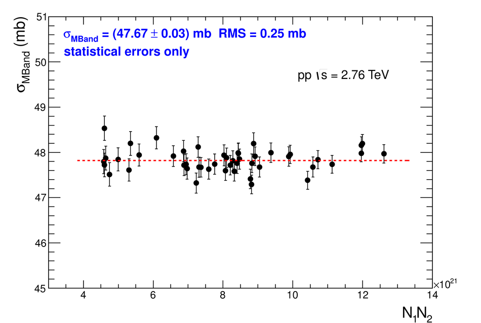
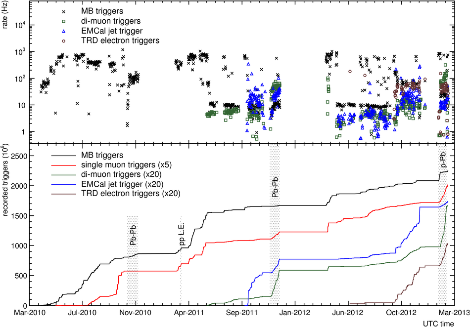
Figure 11
Distribution of the V0 amplitude (sum of V0A and V0C). The centrality bins are defined by integrating from right to left following Eq.(5). The absolute scale is determined by fitting to a model (red line), see below for details. The inset shows a magnified version of the most peripheral region. |  |
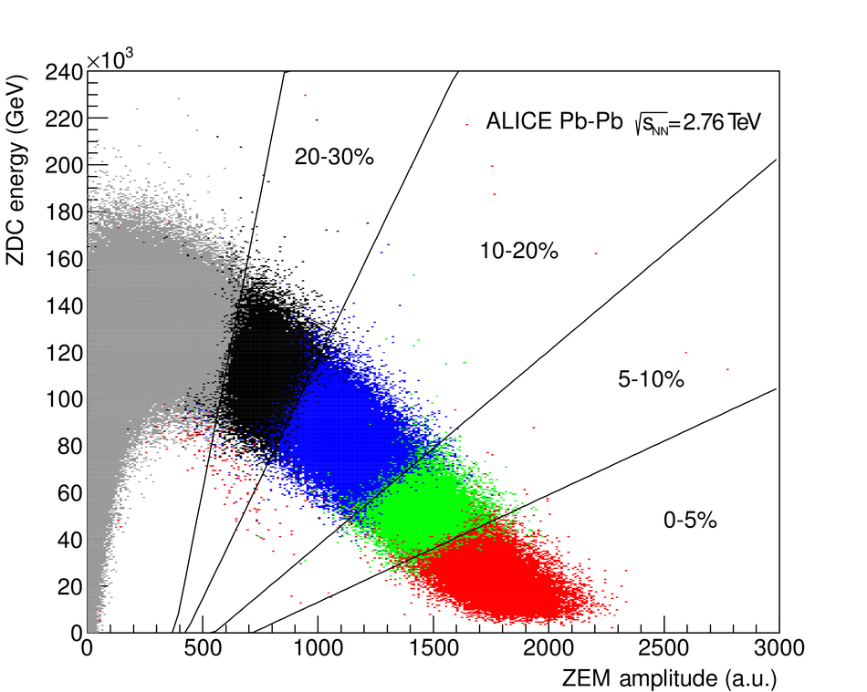
Figure 13
Correlation between signals in the two neutron zero-degree calorimeters. Single electromagnetic dissociation events produce a signal in only one of the calorimeters. Mutual dissociation and hadronic interactions populate the interior of the plot and can be distinguished from each other by the signal in ZEM. | 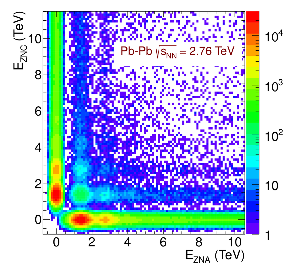 |


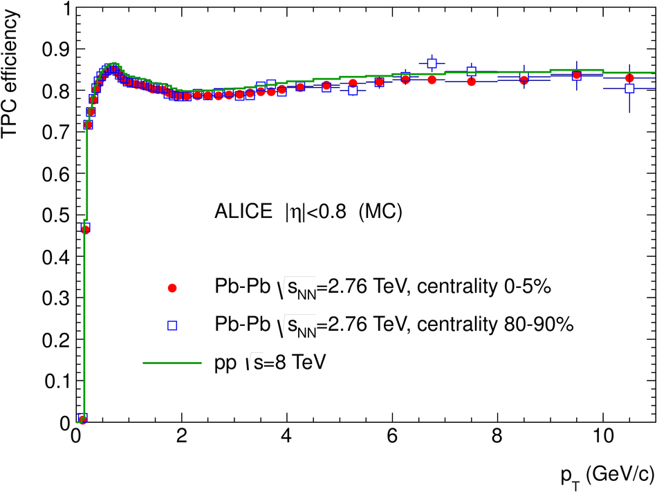
Figure 21
Fraction of reconstructed tracks coming from the primary interaction vertex. Two sets of cuts on the track distance of closest approach ($d_{0}$) to the primary vertex are shown: "loose'' with $|{\rm d}_{0,z}|< 3$ cm, ${\rm d}_{0,xy}< 3$ cm and "strict" with $|{\rm d}_{0,z}|< 2$ cm, ${\rm d}_{0,xy}< (0.0182+0.0350 GeV/c \> \> \pt^{-1}$) cm. | 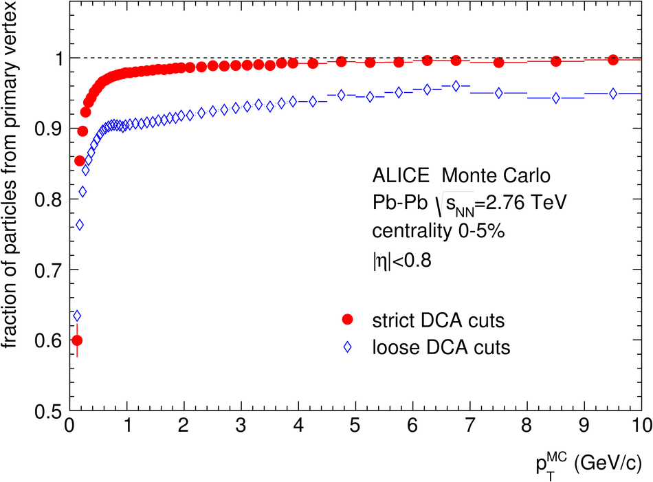 |
Figure 24
Invariant mass spectra of $\mu^+\mu^-$ (top) and $e^+e^-$ (bottom) pairs in ultraperipheral Pb-Pb collisions. The solid and dotted lines represent the background (exponential) and peak (Crystal Ball) fit components, respectively. The bremsstrahlung tail in the $e^+e^-$ spectrum is reproduced in simulation. The mass resolution is better than 1%. |  |
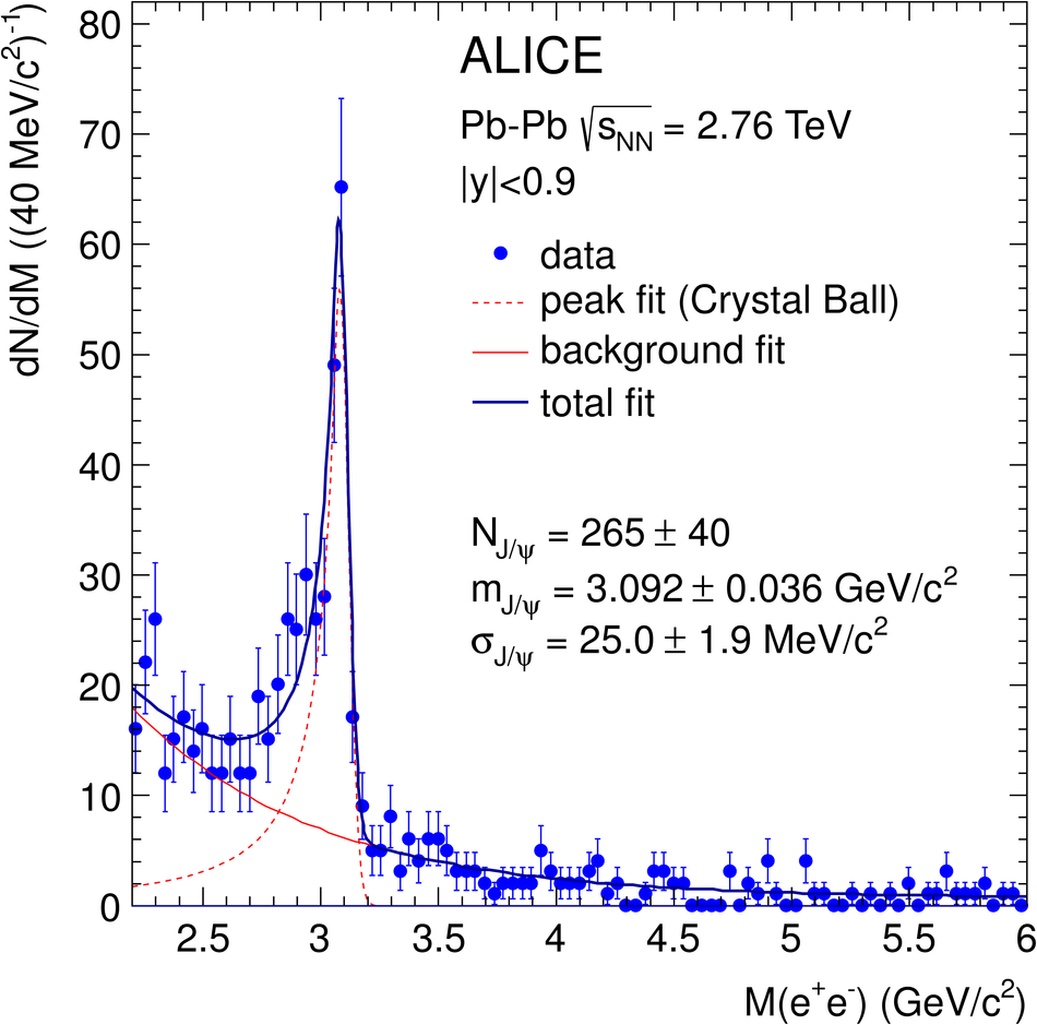
Figure 25
Top: Bunch crossing (BC) ID of tracks obtained from the comparison of time of flight measured in the TOF detector and expected from the track kinematics. The ID is defined with respect to the BC in which the triggering interaction took place The peak at -15 corresponds to tracks not matched in TOF (mostly from the pileup in the TPC, outside of the TOF readout window of 500 ns). Bottom: $z$ coordinates of tracks' PCA to the beam axis in a single event with pileup; the positions of reconstructed vertices with attributed bunch crossings are shown by markers. | 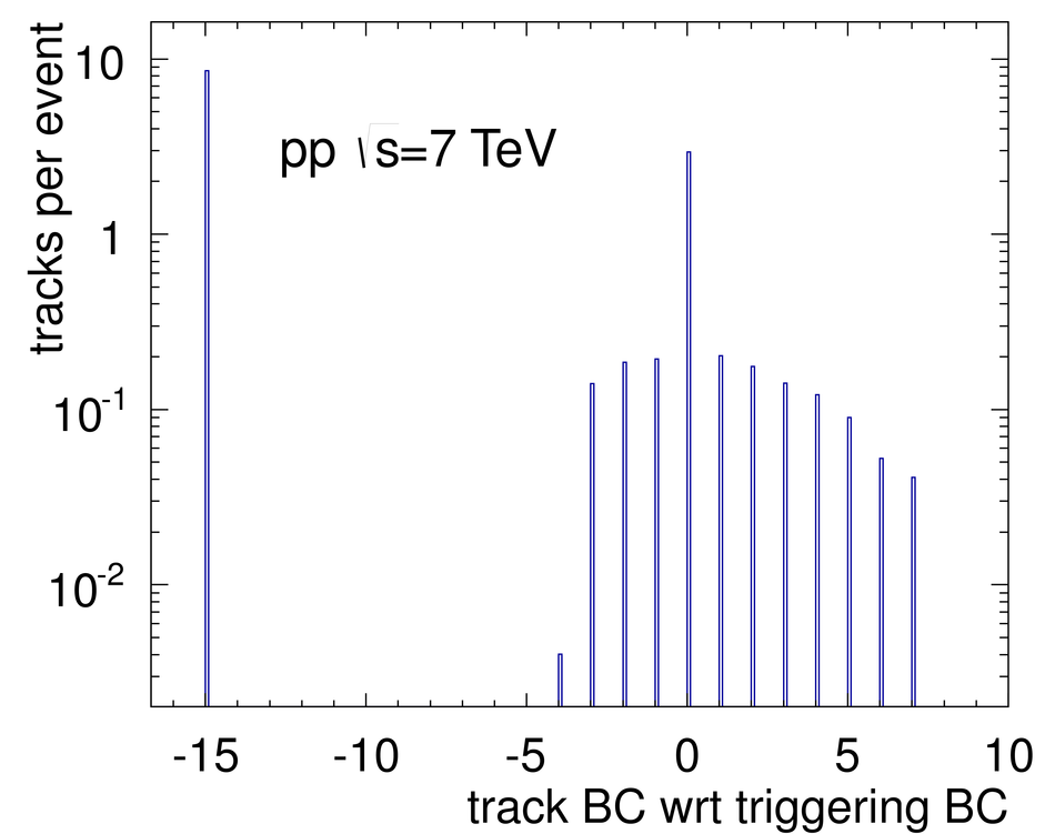 |
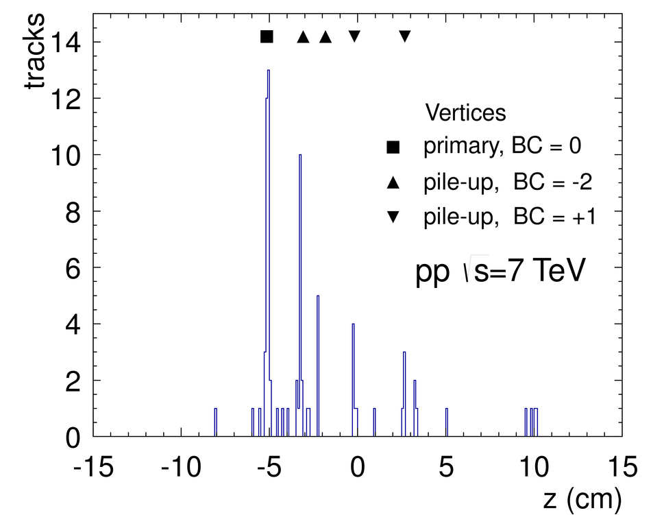
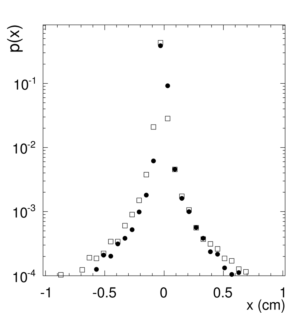
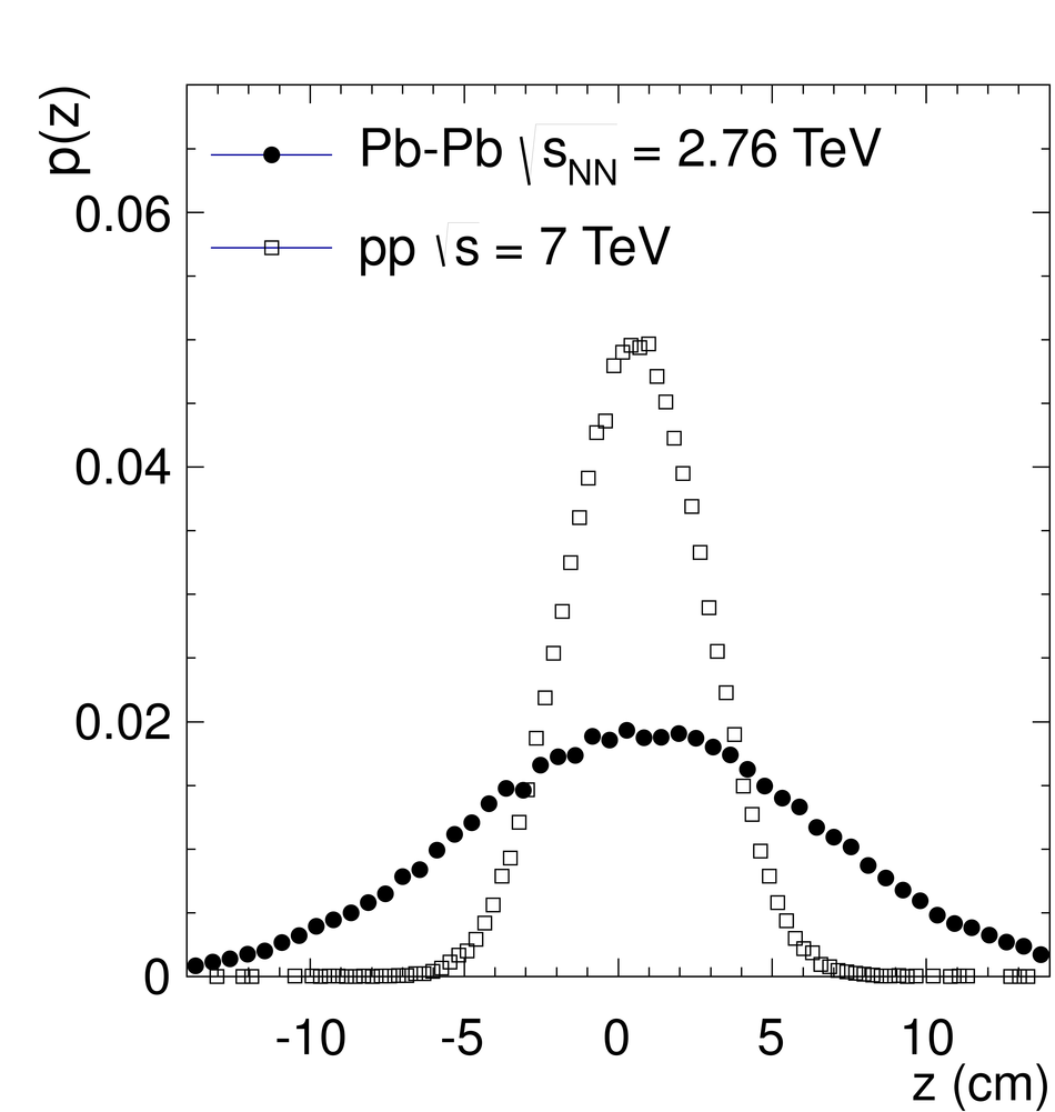
Figure 27
Transverse width of the final vertex distribution (solid points), decomposed into the finite size of the luminous region $\sigma_{D}$ and the vertex resolution $\alpha / \sqrt{(\dNdeta_{ch})^\beta}$ For comparison, the widths of the preliminary (SPD) interaction vertices are shown as open points. | 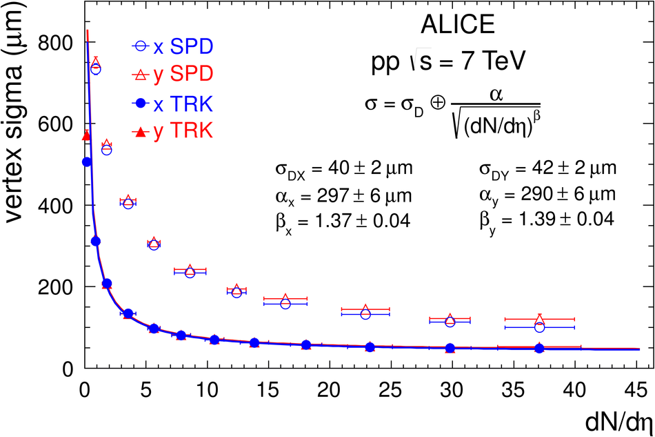 |
Figure 28
Secondary vertex reconstruction principle, with $\Kzs$ and $\Xi^{-}$ decays shown as an example. For clarity, the decay points were placed between the first two ITS layers (radii are not to scale). The solid lines represent the reconstructed charged particle tracks, extrapolated to the secondary vertex candidates. Extrapolations to the primary vertex and auxiliary vectors are shown with dashed lines. | 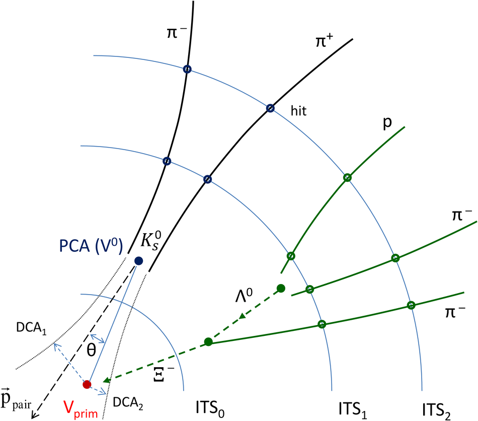 |
Figure 29
Invariant mass distributions of $\pi^+\pi^-$ (left panel) and p$\pi^-$ (middle panel) pairs in central Pb-Pb collisions at $\sNN$ = 2.76 TeV. The hatched areas show the regions of the $\Kzs$ and $\Lambda$ peaks and of the combinatorial background. The right-hand panel shows the reconstruction efficiencies (including the candidate selection cuts) as a function of transverse momentum for central (0-5$\%$) and peripheral (80-90$\%$) collisions. | 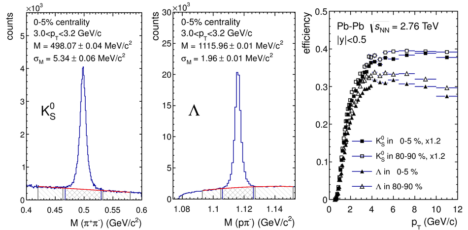 |


Figure 36
Interaction time of the collision with respect to the LHC clock measured by the T0 detector (top) and the resolution of the system obtained as the time difference between T0A and T0C (bottom). The time difference is corrected for the longitudinal event-vertex position as measured by the SPD. | 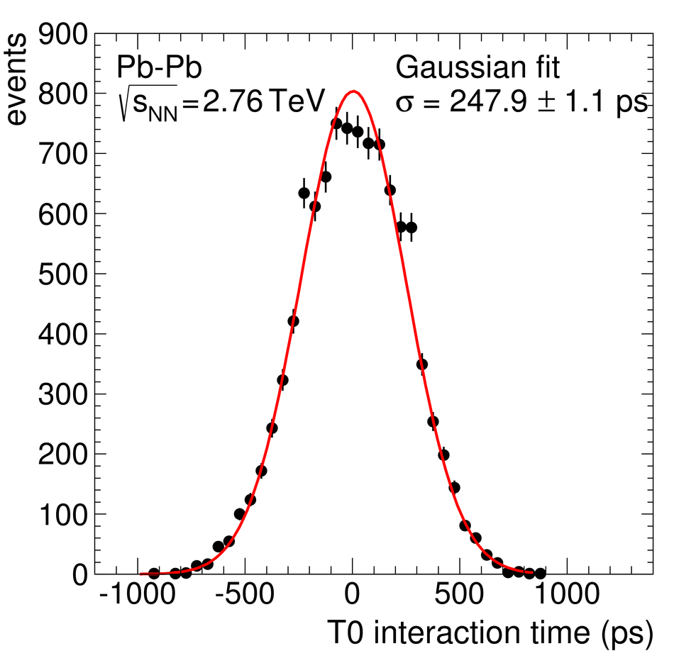 |

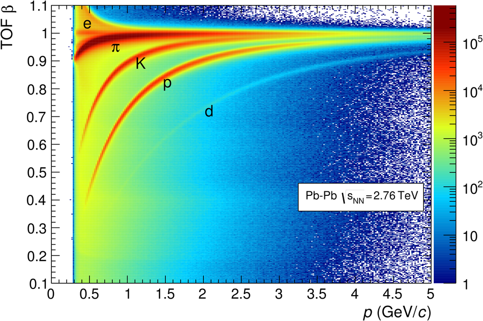
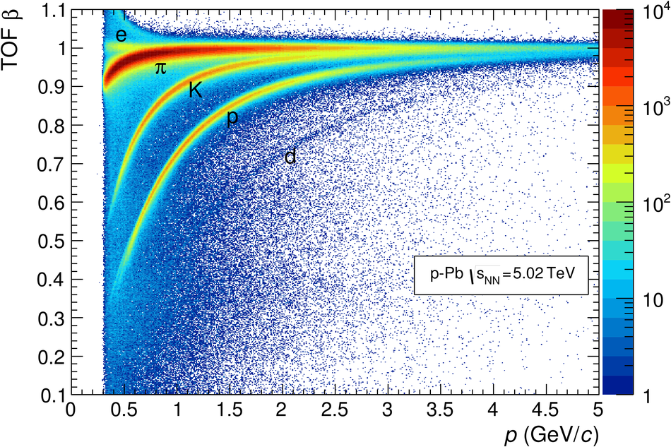
Figure 40
TOF $\beta$ distribution for tracks with momentum 0.95 GeV/$c$ < $p$ < 1.05 GeV/$c$. The Pb-Pb histogram is normalized to the p-Pb one at the pion peak ($\beta=0.99$). While the resolution (width of the mass peaks) is the same, the background of mismatched tracks increases in the high-multiplicity environment of Pb-Pb collisions. Both samples are minimum bias. |  |

Figure 45
Squared particle masses calculated from the momentum and velocity determined with ITS-TPC and HMPID, respectively, in central Pb-Pb collisions at $\sNN$ = 2.76 TeV. The velocity is calculated from the Cherenkov angle measured in the HMPID. Dotted lines indicate the PDG mass values. The pion tail on the left-hand side is suppressed by an upper cut on the Cherenkov angle. The deuteron peak is clearly visible. | 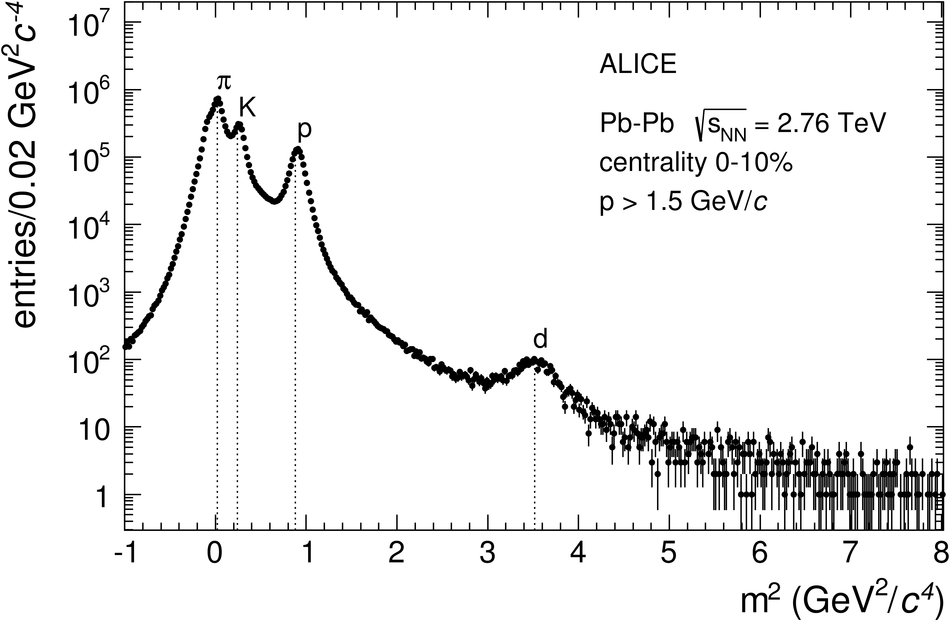 |
Figure 46
Separation power of hadron identification in the ITS, TPC, TOF, and HMPID as a function of $\pt$ at midrapidity. The left (right) panel shows the separation of pions and kaons (kaons and protons), expressed as the distance between the peaks divided by the resolution for the pion and the kaon, respectively, averaged over $|\eta|< 0.5$. For the TPC, an additional curve is shown in a narrower $\eta$ region. The lower panels show the range over which the different ALICE detector systems have a separation power of more than $2\sigma$. | 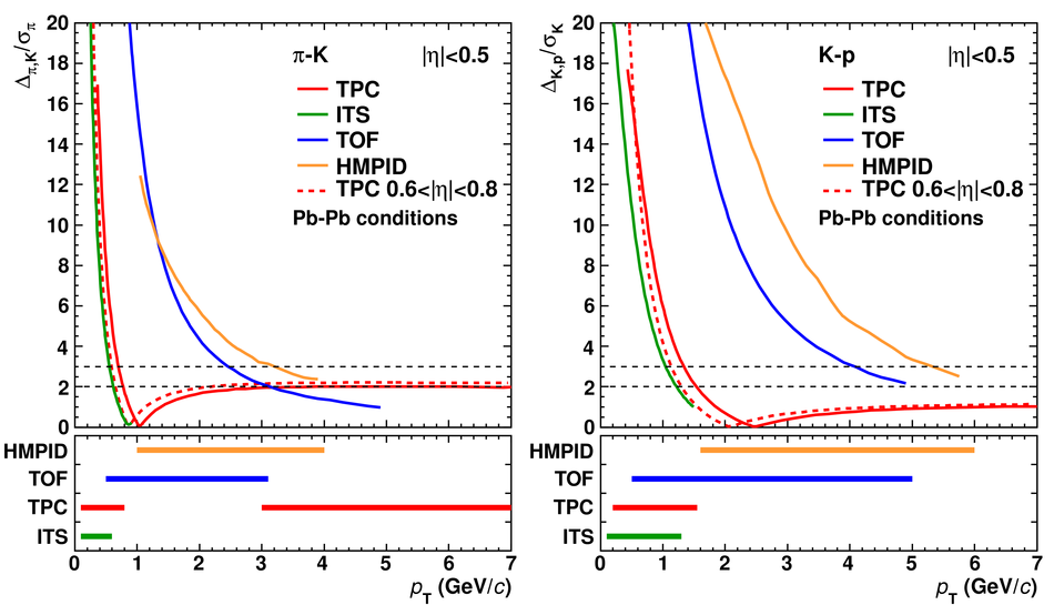 |

Figure 48
Invariant mass of reconstructed charged particles (pions and kaons) decaying inside the TPC volume and producing a secondary vertex (kink). The mass is calculated assuming that the track segment after the kink represents a muon and that the neutral decay daughter is a neutrino. The neutrino momentum is taken from the difference between the momenta of the track segments before and after the kink. | 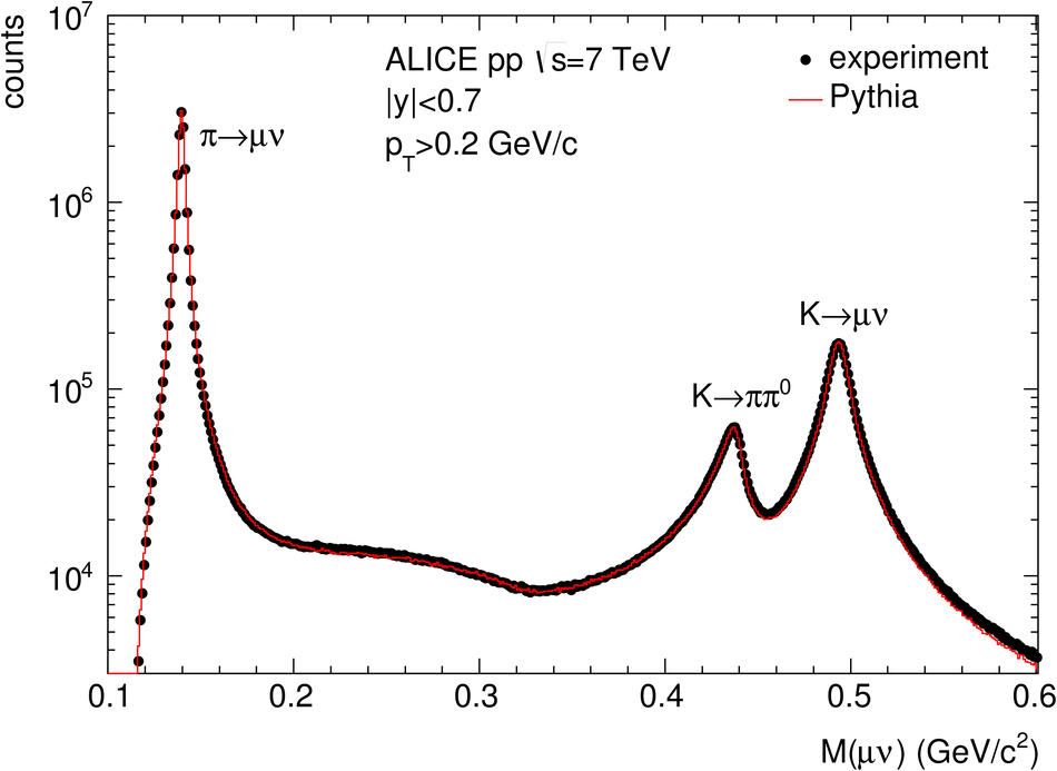 |

Figure 51
Measured $dE/dx$ signal in the ALICE TPC versus magnetic rigidity, together with the expected curves for negatively-charged particles. The inset panel shows the TOF mass measurement which provides additional separation between$^3\overline{\rm He}$ and $^4\overline{\rm He}$ for tracks with $p/Z > 2.3$ GeV/$c$. | 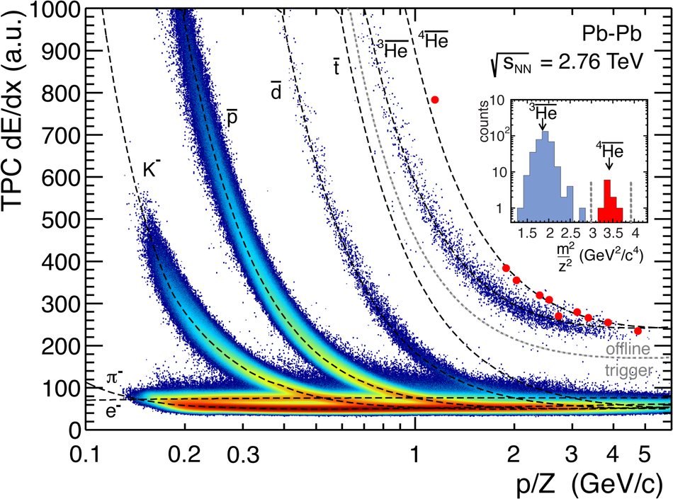 |
Figure 52
Distribution of the residuals forthe EMCal clusters to track matching in pseudorapidity ($\eta_{\rm cluster}-\eta_{\rm track}$) vs. azimuth ($\phi_{\rm cluster}-\phi_{\rm track}$) in pp collisions at $\sNN$ = 7 TeV triggered by EMCal. Only clusters with an energy $E_{\rm cluster}>1$ GeV and tracks with a transverse momentum $p_{\rm T, track}>1$ GeV/$c$ are used. | 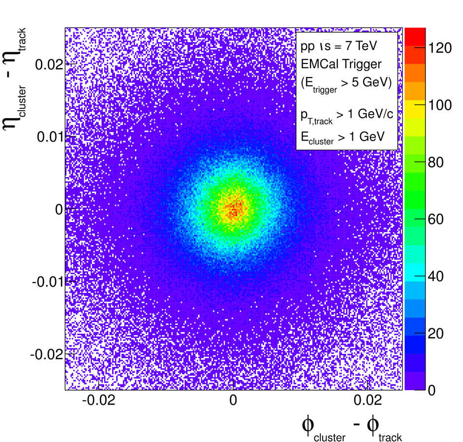 |
Figure 53
$E/p$ distributions for (a) electrons and (b) pions in pp collisions at $\sqrt{s}$ = 7 TeV, measured in the experiment (reddotted line), and compared to simulation (black full line). The samples of identified electrons and pions were obtained from reconstructed$\gamma$ conversions and $\Lambda$/$\Kzs$ decays, respectively. The simulation is a Pythia simulation with realistic detector configuration and full reconstruction. |  |
Figure 54
Relative resolution of $E/p$ vs. transverse momentum $\pt$ for electrons in experimental data (full dots) and from a fully reconstructed MC (open circles) in pp collisions at $\sqrt{s}$ = 7 TeV. The EMCal energy resolution deduced from the width of the ${\rm \pi^0}$ and $\eta$ invariant mass peaks (black dotted line), added in quadrature to the TPC $\pt$ resolution (green dash-dotted line), describes the measurement reasonably well (red solid line). | 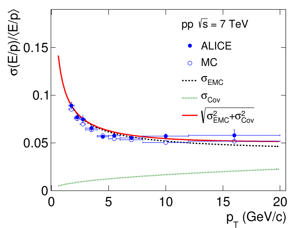 |

Figure 58
Pion efficiency as a function of electron efficiency (top panel,for 6 layers) and as a function of the number of layers (bottom panel, for 90% electron efficiency) for the momentum range 0.9-1.1 GeV/$c$. The results are compared for the truncated mean, LQ1D, LQ2D, and NN methods. | 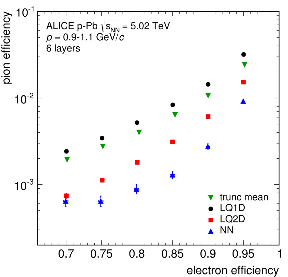 |
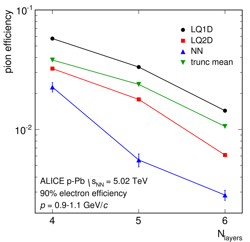
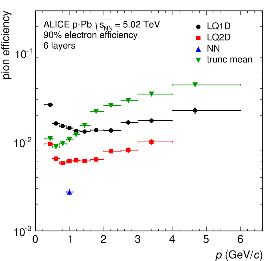
Figure 61
Invariant mass distribution for $\jpsi$ candidates from EMCal-triggered events in pp collisions at $\sqrt{s}$ = 7 TeV ($\mathcal{L} \approx 0.4$ pb$^{-1}$, 8M events). Electrons are identified by their energy loss in the TPC ($dE/dx$ > 70) and the $E/p$ ratio in the EMCal ($0.9< E/p< 1.1$) for both legs. A fit to the signal(Crystal Ball [50]) and the background (exponential) is shown in addition. | 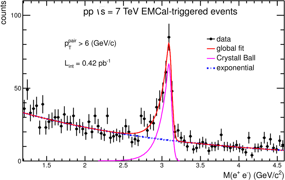 |
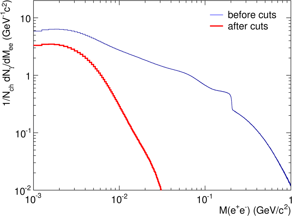

Figure 67
Radial distribution of the reconstructed photon conversion points for $|\eta|< 0.9$ (black) compared to MC simulations performed with PHOJET (red). Distributions for true converted photons are shown in yellow. Physics contamination from true ${\rm \pi^0}$ and $\eta$ Dalitz decays, where the primary $e^+e^-$ are reconstructed as photon conversions, are shown as dashed blue histograms. Random combinatorics and true hadronic background are also shown. | 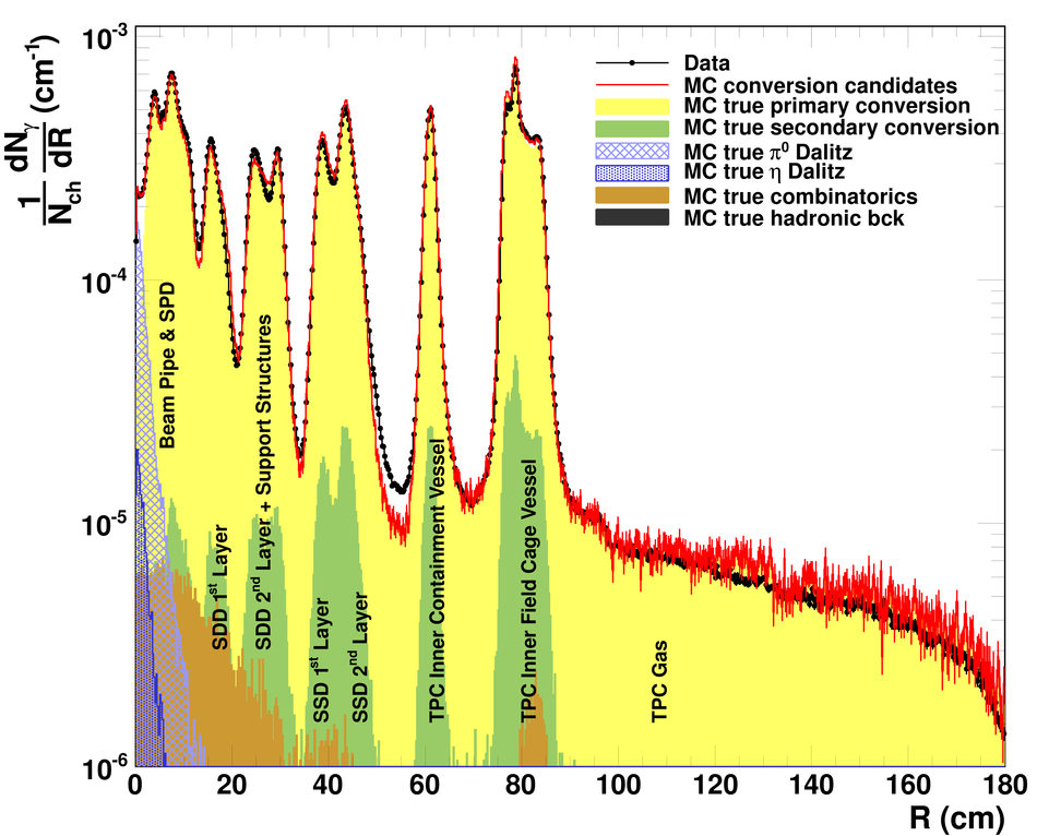 |
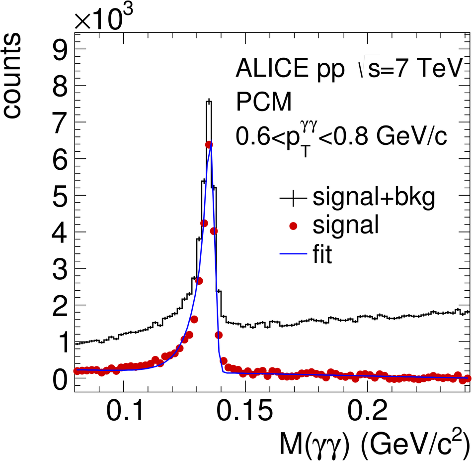
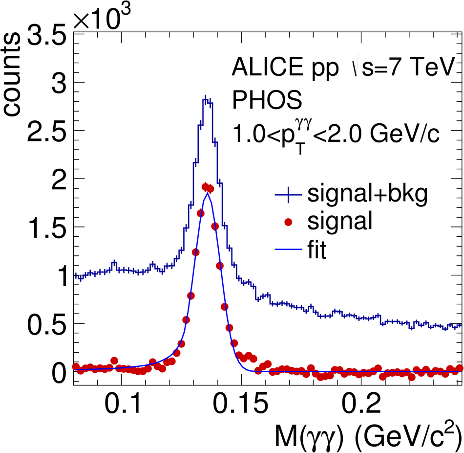
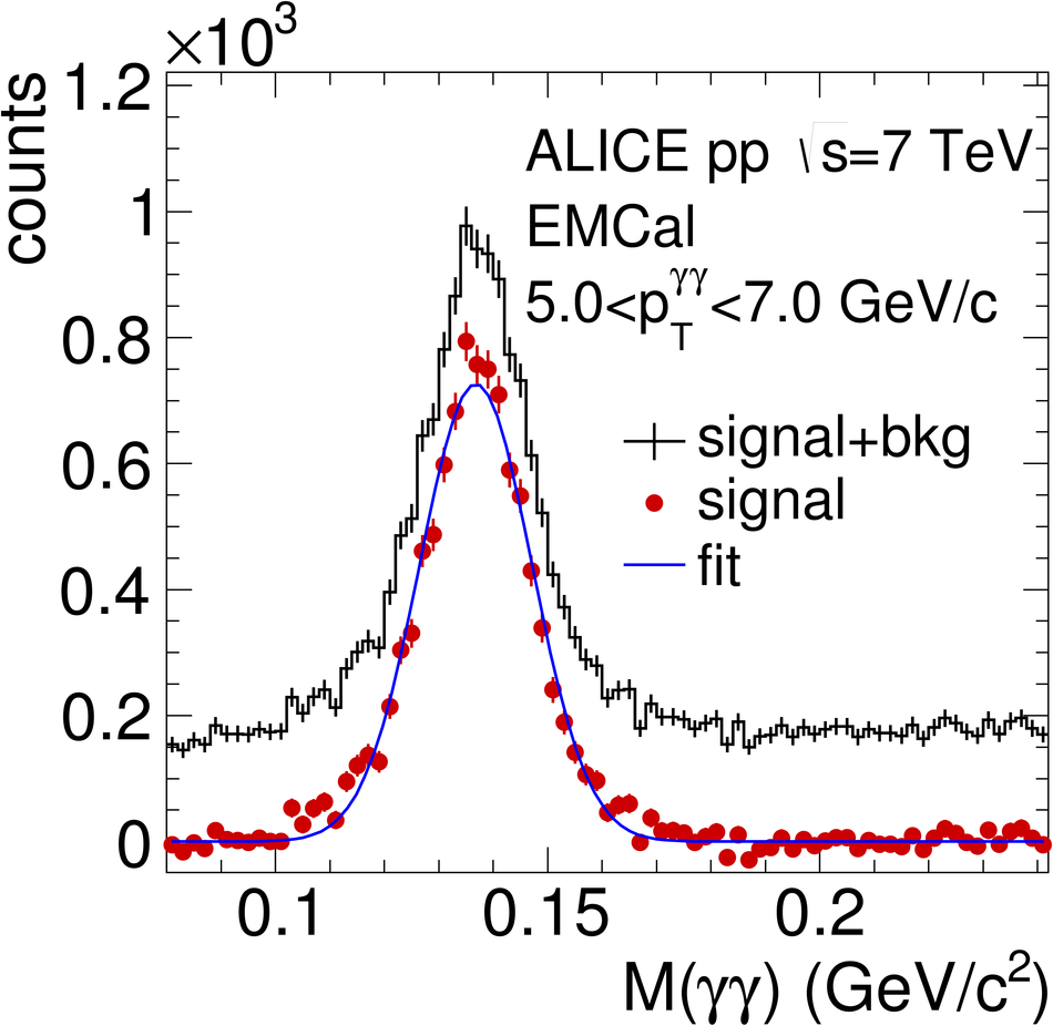

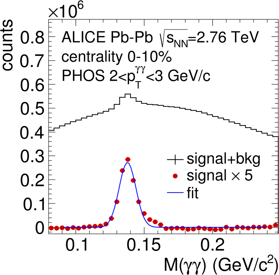
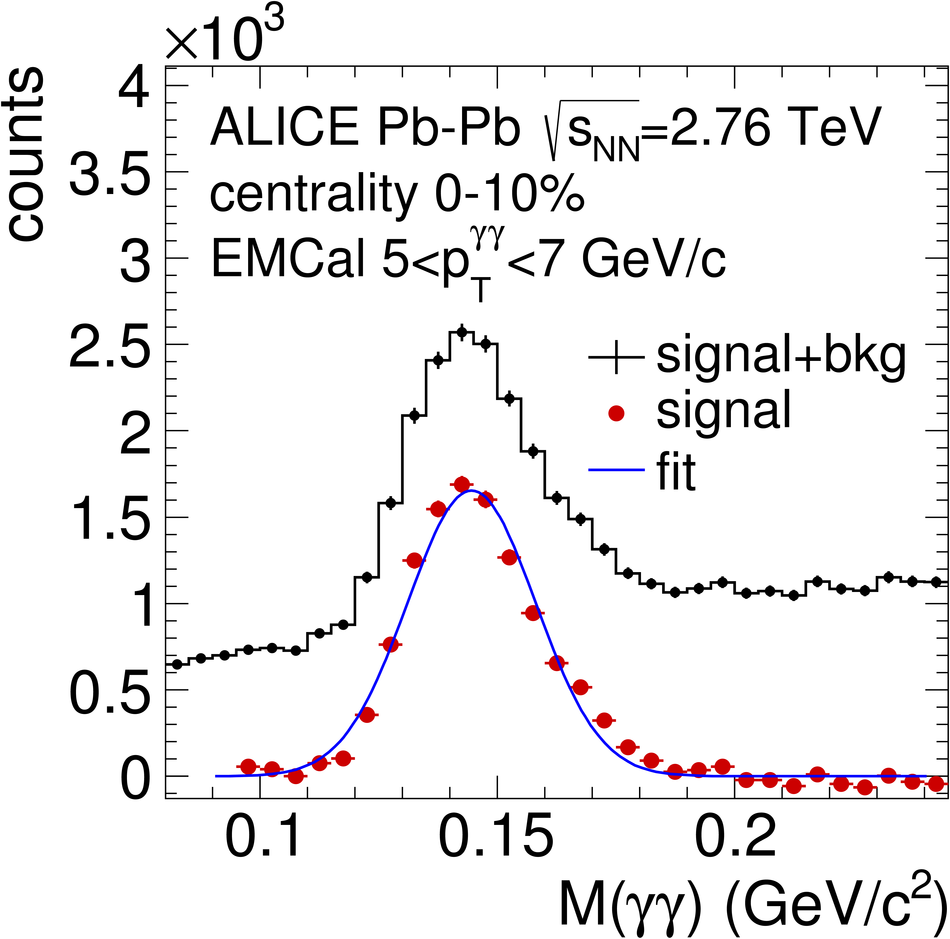
Figure 72
Total correction (efficiency and acceptance) for $|y|< 0.5$ for ${\rm \pi^0}$ reconstruction via two-photon invariant mass determination in pp collisions at $\sqrt{s}$ = 7 TeV (top panel) and in 0-10% central Pb-Pb collisions at $\sNN$ = 2.76 TeV (bottom panel) for PCM, PHOS, and EMCal. | 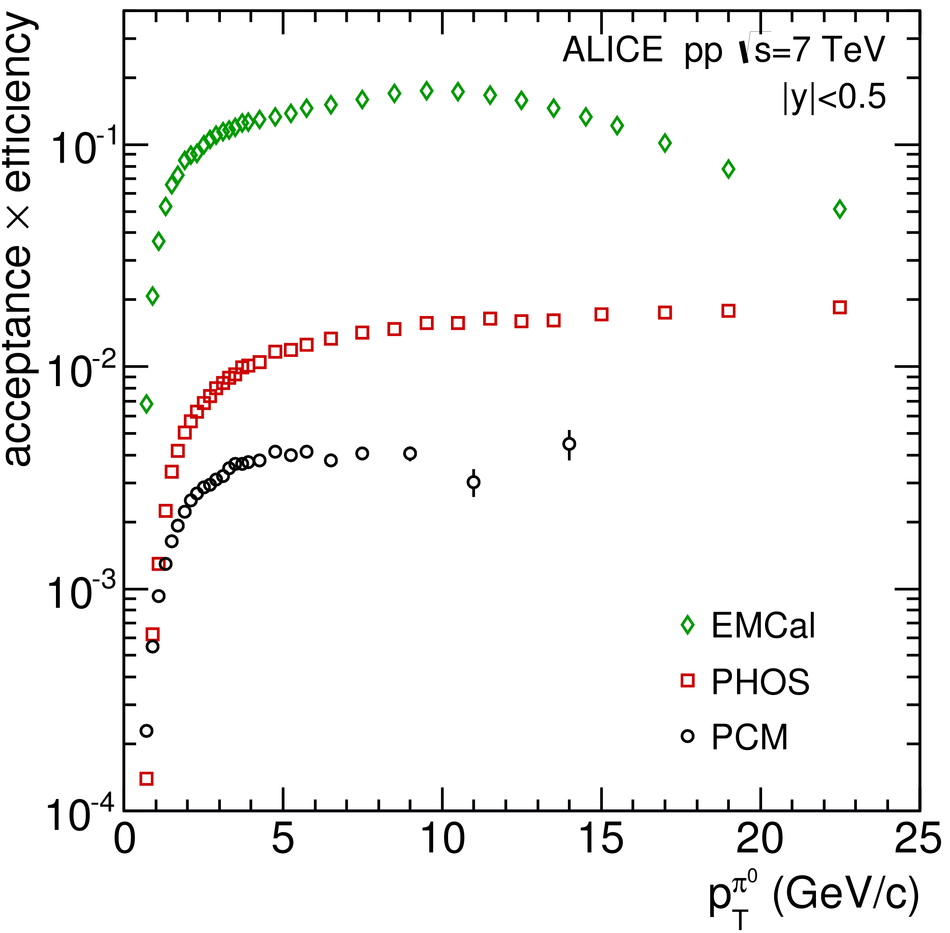 |
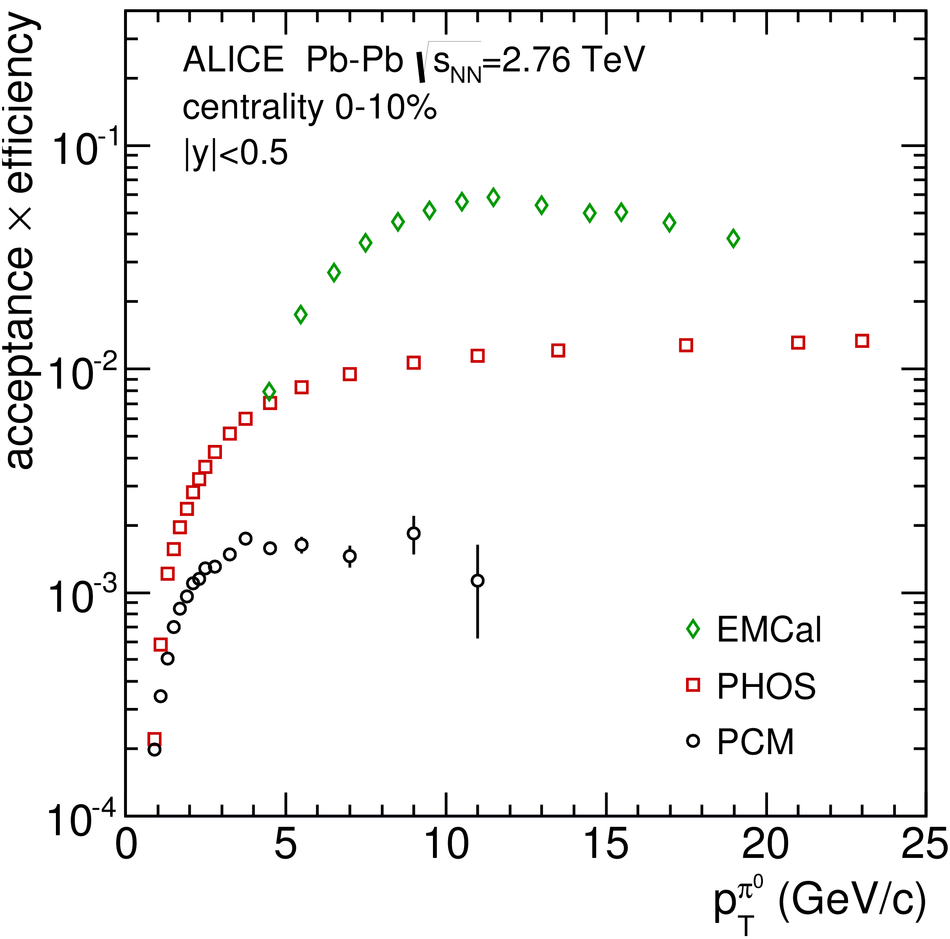
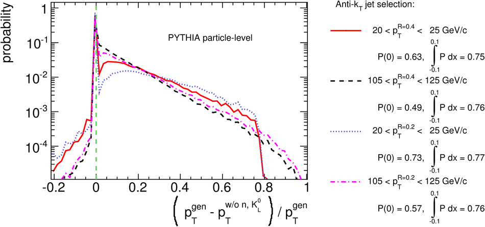
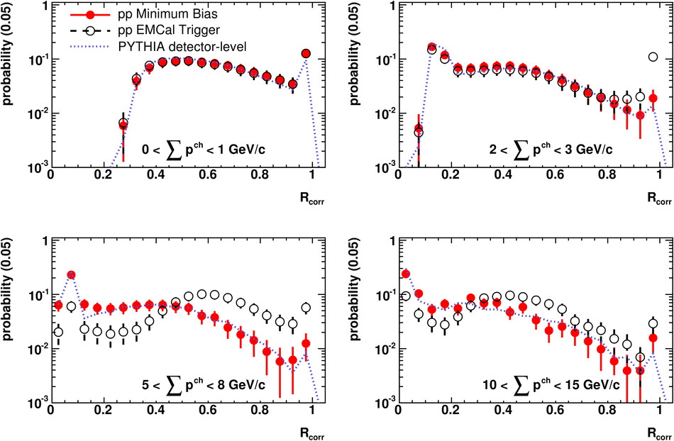
Figure 76
Mean transverse momentum, $\left< \pt\right>$, of constituents measured in reconstructed jets in 2.76 TeV pp collisions (anti-$\kT$, $R=0.4$) vs. jet $\pt$. Left: charged tracks; Right: neutral clusters. Data are shown for MB and SSh triggers, and are compared to detector-level simulations. | 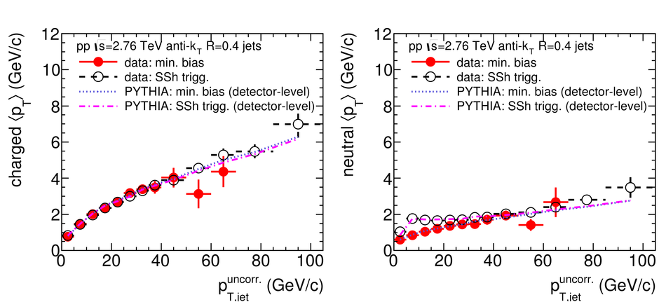 |
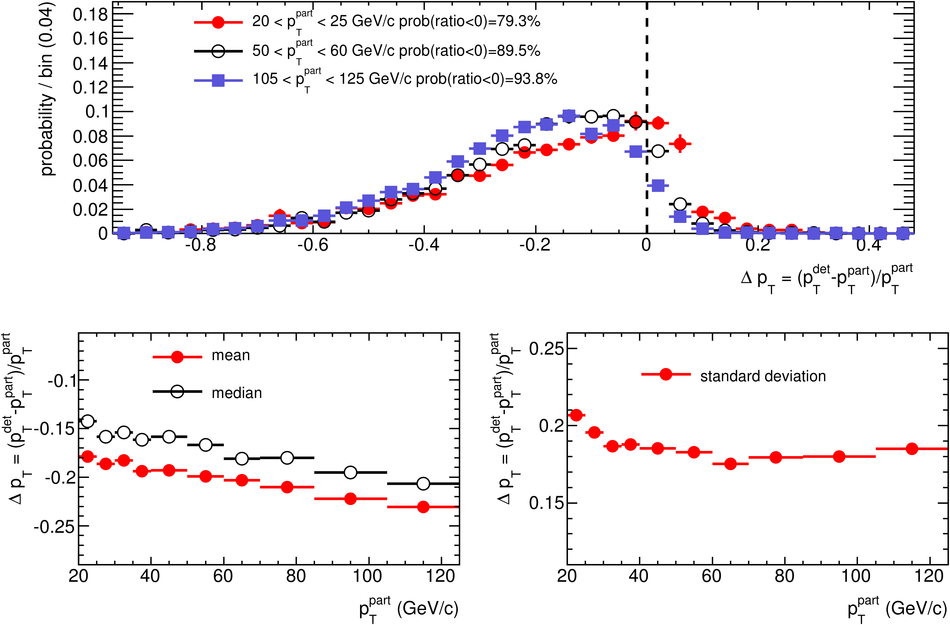
Figure 80
Probability distribution of $R_{\rm corr}$ (Eq. (18)) in two different intervals of $\sum_p$, measured in central (0-10%) and peripheral (70%-80%, left panel only) Pb-Pb collisions. Also shown are detector-level simulations for MB pp collisions based on PYTHIA (same distributions as Fig. 75), and for central PbPb collisions based on HIJING (left panel only). | 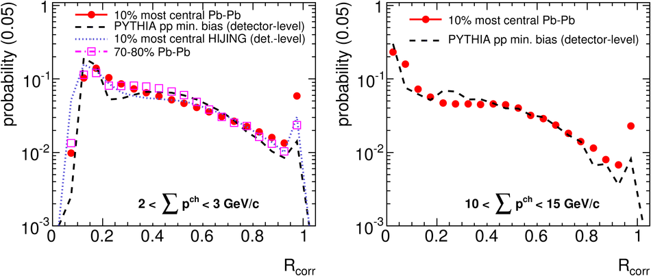 |
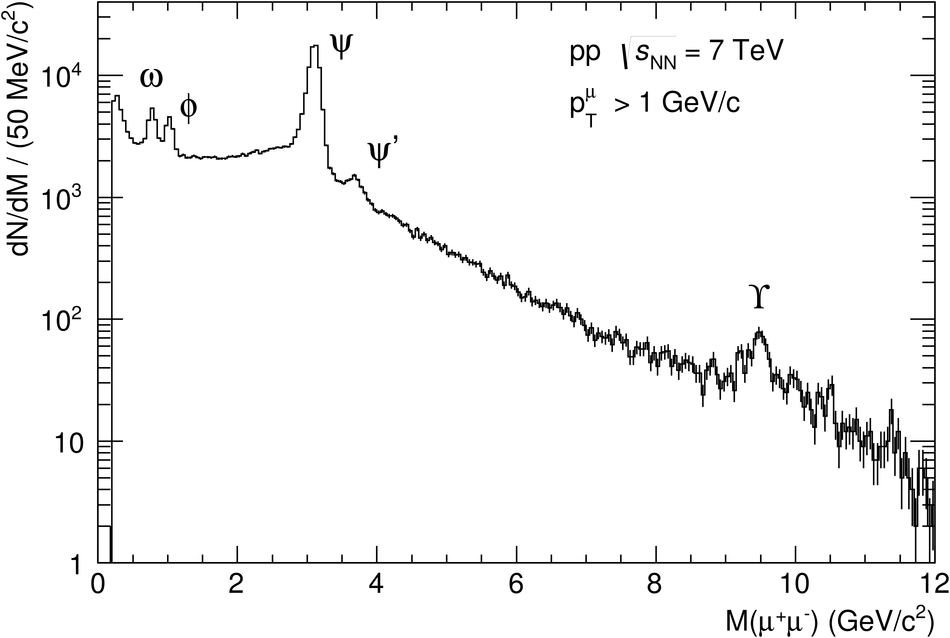
Figure 87
Invariant-mass distribution of $\mu^+ \mu^-$ pairs in Pb-Pb collisions at $\sNN$ = 2.76 TeV with the $\Upsilon(1S)$, $\Upsilon(2S)$, and $\Upsilon(3S)$ peaks fitted by the sum of three extended Crystal Ball functions with identical relative widths and identical relative displacements from the PDG mass values. The tail shape is fixed by the embedding-MC simulation and the combinatorial background is parametrized by an exponential. | 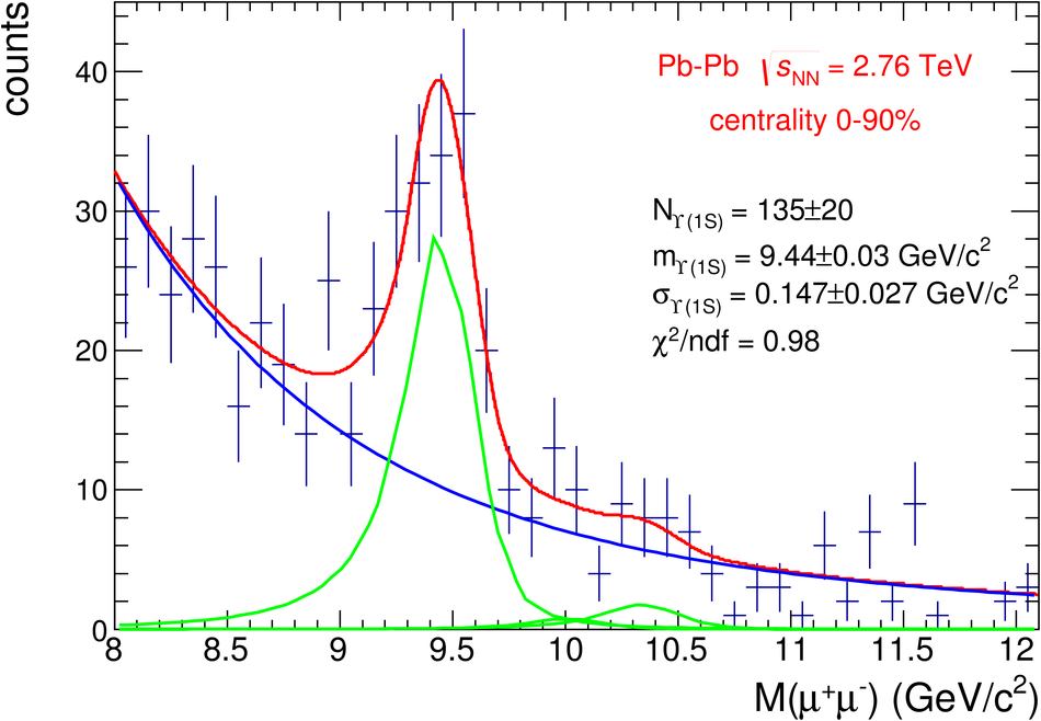 |
![[png]](https://alice-publications.web.cern.ch/sites/default/files/papers/716/ITS_TPC_trackingEff_pp-8426.png)
![[png]](https://alice-publications.web.cern.ch/sites/default/files/papers/716/ITS_TPC_trackingEff_PbPb-8427.png)
![[png]](https://alice-publications.web.cern.ch/sites/default/files/papers/716/TRD_Performance_logo0_pid1-8552.png)