The production of mesons containing strange quarks (K0s, phi) and both singly and doubly strange baryons (Lambda, Anti-Lambda, and Xi+Anti-Xi) are measured at central rapidity in pp collisions at $\sqrt{s} = 0.9$ TeV with the ALICE experiment at the LHC. The results are obtained from the analysis of about 250 k minimum bias events recorded in 2009. Measurements of yields (dN/dy) and transverse momentum spectra at central rapidities for inelastic pp collisions are presented. For mesons, we report yields ($\left< dN/dy\right>$) of $0.184 \pm 0.002 (stat.) \pm 0.006 (syst.)$ for K0s and $0.021 \pm 0.004 (stat.) \pm 0.003 (syst.)$ for phi. For baryons, we find $<dN/dy> = 0.048 \pm 0.001 (stat.) \pm 0.004 (syst.)$ for $Lambda$, $0.047 \pm 0.002 (stat.) \pm 0.005 (syst.)$ for Anti-Lambda and $0.0101 \pm 0.0020 (stat.) \pm 0.0009 (syst.)$ for Xi+Anti-Xi. The results are also compared with predictions for identified particle spectra from QCD-inspired models and provide a baseline for comparisons with both future pp measurements at higher energies and heavy-ion collisions.
Eur. Phys. J. C 71 (2011) 1594
HEP Data
e-Print: arXiv:1012.3257 | PDF | inSPIRE
CERN-PH-EP-2010-065
Figure 1
Primary vertex distributions for the analyzed events The left panel shows the distributions along the beam axis. Selected events (full symbols) are required to have a reconstructed primary vertex with $|z|< 10 cm$ The right panel corresponds to the directions perpendicular to the beam axis: horizontally(i.e. $x$-direction, squares and full line) and vertically (i.e. $y$-direction, triangles and dashed line). | 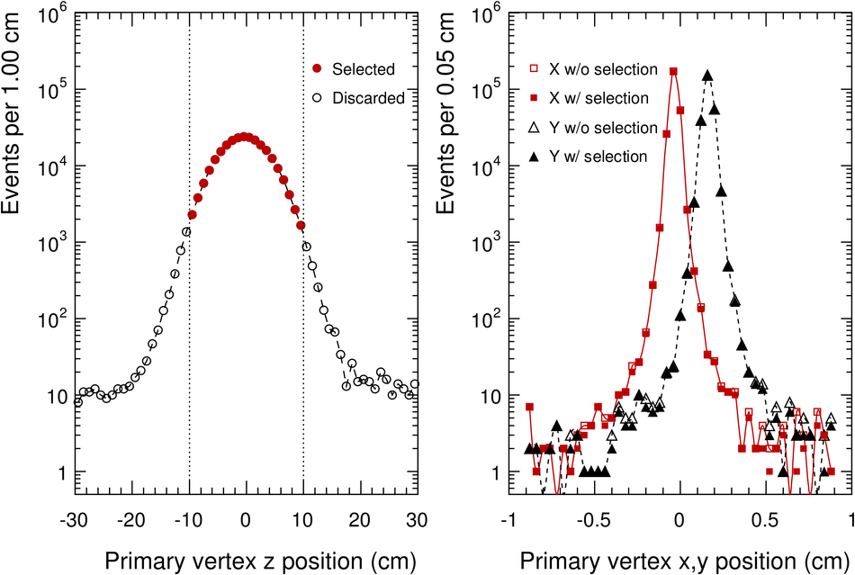 |
Figure 3
Armenteros-Podolanski distribution for V0 candidates showinga clear separation between $\Kzs$, $\mathrm {\Lambda}$ and $\mathrm {\overline{\Lambda}}$ The $\gamma$ converting to $e^{+}e^{-}$ with the detector material arelocated in the low $q_{T}$ region, where $q_{T}$ is the momentum componentperpendicular to the parent momentum vector. |  |
Figure 4
$\Kzs$, $\mathrm {\Lambda}$ and $\mathrm {\overline{\Lambda}}$ lifetime distributions obtained for the candidates selected by the invariant mass within a $\pm 3\sigma$ region around the nominal mass and corrected for detection efficiency The distributions are scaled for visibility and fitted to an exponential distribution (straight lines) Only statistical uncertainties are shown. | 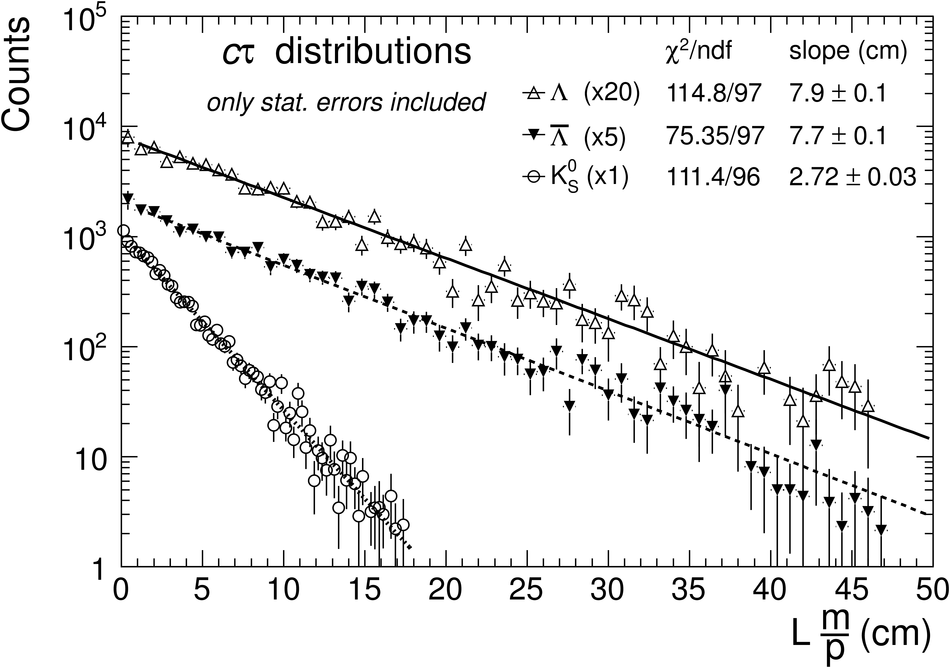 |
Figure 5
Left panel shows the distribution of the measured energy-deposit of charged particles versus their momentum in the TPC The dashed lines delimit successively a $\pm 5\sigma$ then a $\pm 3\sigma$ selection of the kaon tracks using the ALEPH parameterization of the Bethe-Bloch curve (solid line) Right panel shows the relative difference between TOF measured times and that corresponding to a kaon mass hypothesis The dashed lines delimit a coarse fiducial region compatible with this kaon hypothesis. | 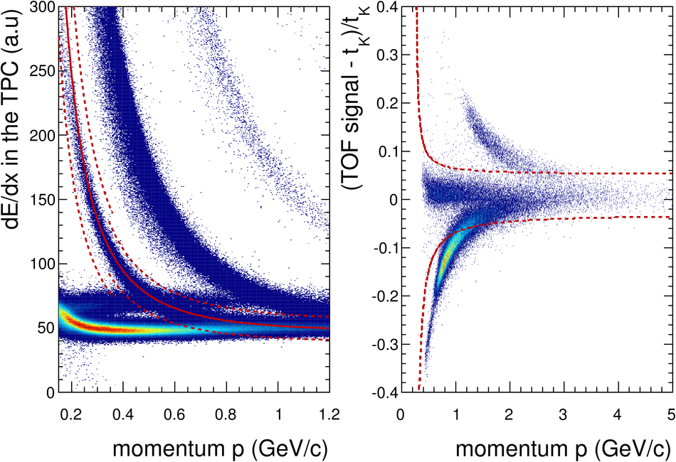 |
Figure 6
Plot illustrating the "bin-counting" method used to extract the raw yields It corresponds to the invariant mass distribution of $\Kzs$ for the $\pT$ bin $[0.4-0.5] $GeV/c The hashed regions show where the background is sampled; they are chosen to be $6\sigma$ away from the signal approximated with a Gaussian distribution The averaged or fitted background is subtracted from the signal region of $\pm 4\sigma$. |  |
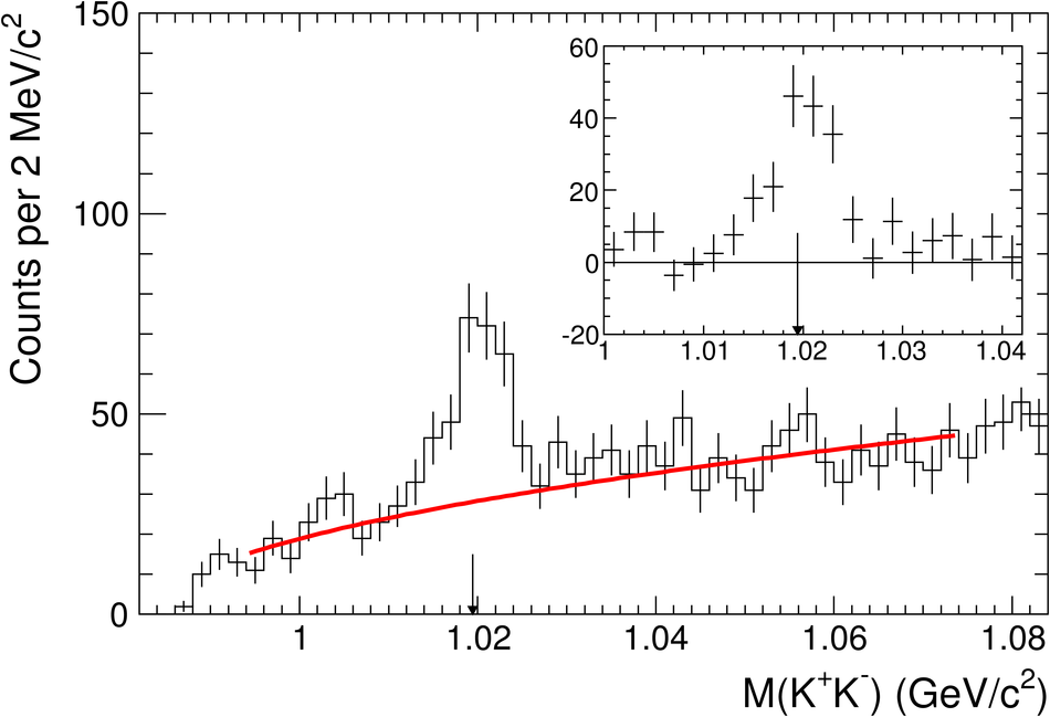
Figure 8
Reconstructed (raw) yields of $\Kzs$ (open circles), $\mathrm {\Lambda}$ (open squares)and $\mathrm {\overline{\Lambda}}$ (open triangles) as a function of $\pT$. The change of bin size results in successive offsets of the raw counts at $\pT = [1.4, 1.6, 2.4] $GeV/c for $\Kzs$ and$\pT = [1.6, 2.4, 3.0] $GeV/c for $\mathrm {\Lambda}$ and $\mathrm {\overline{\Lambda}}$ Uncertainties correspond to the statistics and the systematics from the signal extraction They are represented by the vertical error bars. The horizontal error bars give the bin width. | 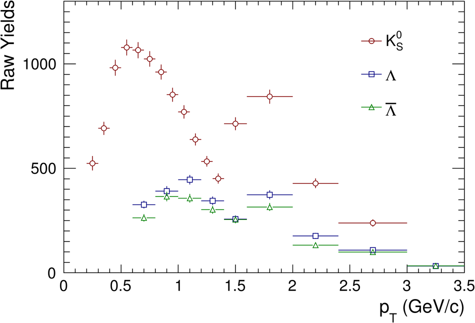 |
Figure 9
Reconstructed (raw) yields of $\phi$ (stars) and $\mathrm {\Xi^{-}+\overline{\Xi}^{+}}$ (diamonds) as a function of $\pT$ With the current statistics, 4$ \pT$ bins are used for the $\phi$ ([0.7-1.0], [0.7-1.5], [1.5-2.0]and [2.0-3.0]$ $GeV/c) and $3 \pT$ bins for the $\mathrm {\Xi^{-}+\overline{\Xi}^{+}}$ ([0.6-1.4], [1.4-2.0] and [2.0-3.0]$ $GeV/c) Uncertainties correspond to the statistics (i.e. the number of reconstructed particles)and the systematics from the signal extraction. They are represented by the vertical error bars(the horizontal ones give the bin width). | 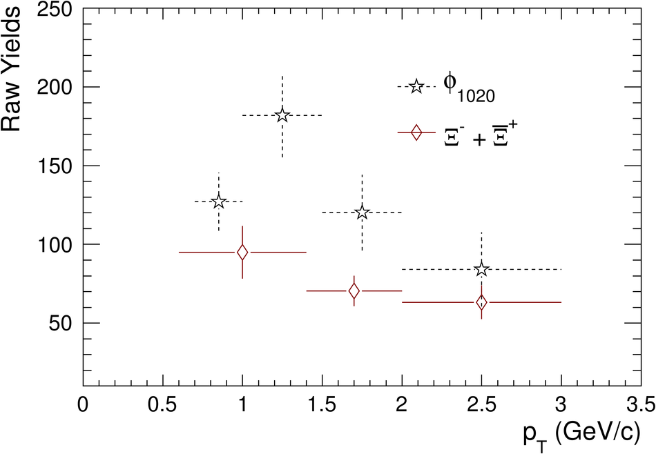 |
Figure 10
Efficiency of $\Kzs$ (open circles), $\mathrm {\Lambda}$ (open squares) and $\mathrm {\overline{\Lambda}}$(open triangles) as a function of $\pT$ The uncertainties correspond to the statistics in Monte Carlo samples used to compute thecorrections The efficiency is limited by the branching ratio represented by a solid arrow for $\Kzs$ (0.692)and by a dashed arrow for $\mathrm {\Lambda}$ and $\mathrm {\overline{\Lambda}}$ (0.639) . | 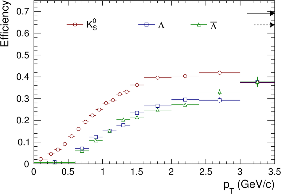 |
Figure 11
Efficiency of $\phi$ (stars) and $\mathrm {\Xi^{-}+\overline{\Xi}^{+}}$ (diamonds)as a function of $\pT$. The uncertainties correspond to the statistics in the Monte Carlo sample used to compute the corrections The efficiency is limited by the branching ratio represented by a solid arrow for $\mathrm {\Xi^{-}+\overline{\Xi}^{+}}$ (0.636)and by a dashed arrow for $\phi$ (0.492) |  |
Figure 12
Comparison between data (red circles) and Monte Carlo (black open triangles)for several topological variables used to select secondary vertices. Thetop panels correspond tothe $\Kzs$ candidates selected in a $\pm 20 $MeV$/c^2$ invariant mass window around the nominal mass The distribution of the DCA between the positive daughter track and the primary vertex and the DCA distribution between the two daughters tracks are displayed in the left and the right top panels respectively. On the bottom panels, the same distributions are shown for the $\mathrm {\overline{\Lambda}}$ candidates selected in a $\pm 8 $MeV$/c^2$ invariant mass window around the nominal mass. |  |
Figure 13
Comparison of the corrected yields as a function of $\pT$ for $\Kzs$ (circle) and charged kaons ($\mathrm{K^{+}}$) (open squares), identified via energy loss in the TPC and ITS, and via time of flight in the TOF The points are plotted at the centre of the bins The full vertical lines associated to the $\Kzs$ points, as well as the gray shaded areas associated to the $\mathrm{K^{+}}$ points, correspond to the statistical and systematic uncertainties summed in quadrature whereas the inner vertical lines contain only the statistical uncertainties (i.e. the number of reconstructed particles) and the systematics from the signal extraction. |  |
Figure 14
Particle spectra (corrected yields) as a function of $\pT$ for $\Kzs$ (circles),$\mathrm {\Lambda}$ (squares), $\mathrm {\overline{\Lambda}}$ (triangles), $\phi$ (stars) and $\mathrm {\Xi^{-}+\overline{\Xi}^{+}}$ (diamonds). The data points are scaled for visibility and plotted at the centre of the bins Uncertainties corresponding to both statistics (i.e. the number of reconstructed particles)and systematics from the signal extraction are shown as vertical error bars Statistical uncertainties and systematics (summarized in Table 4) added in quadrature are shown as brackets The fits (dotted curves) using $L\grave{e}vy$ functional form [see Eq.2] are superimposed \begin{align*} &(2)& \frac{d^{2}N}{dyd\pT} & = & \frac{(n-1)(n-2)} {nT [nT + m(n-2)]} \times \frac{dN}{dy} \times \pT \times \left( 1+ \frac{m_{\rm T}-m}{nT}\right)^{-n} \end{align*} |  |
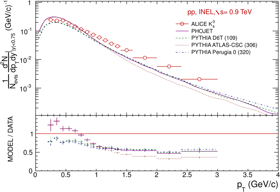
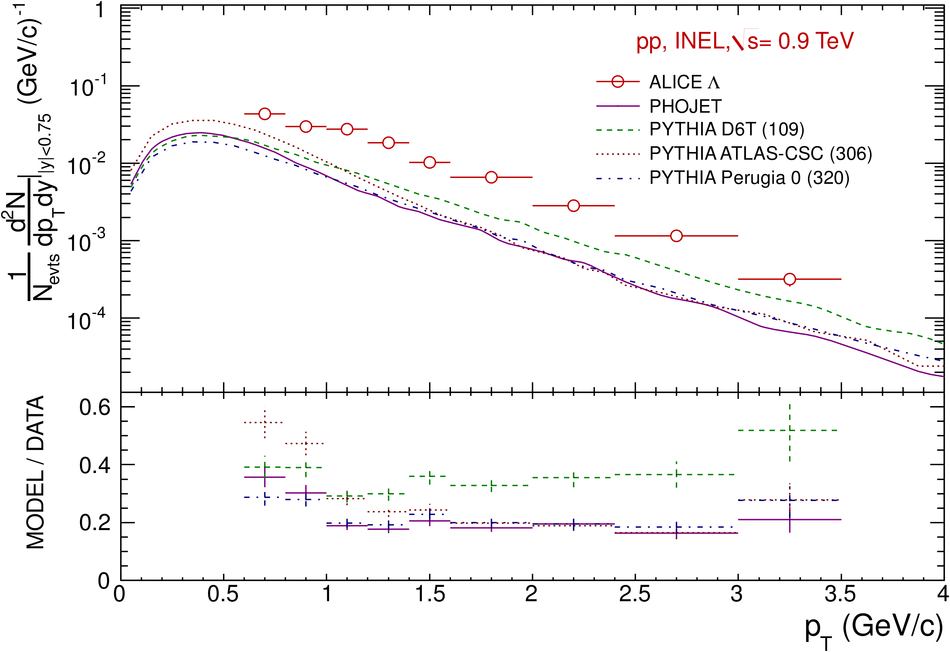

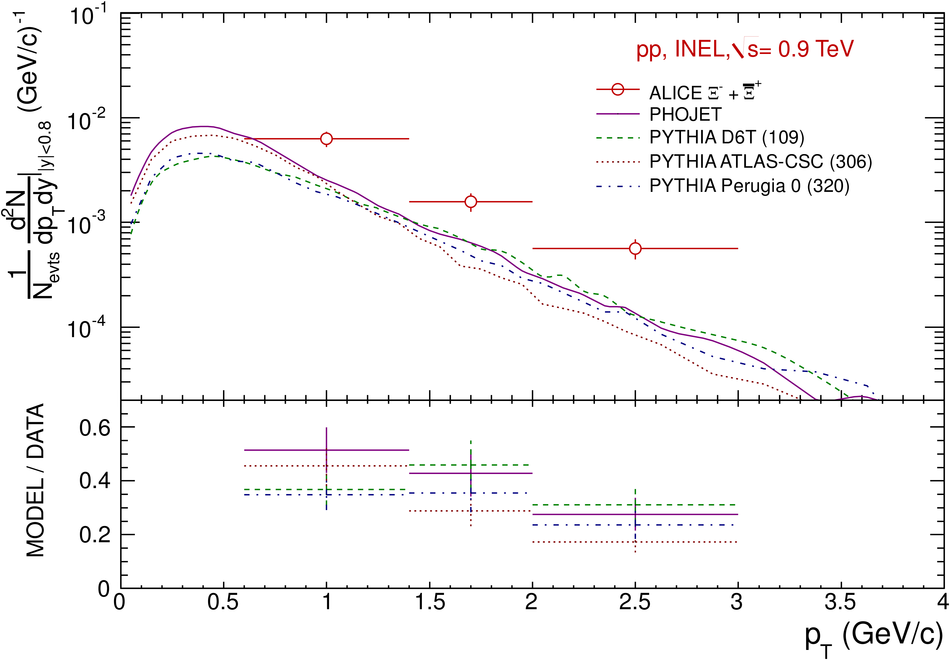
Figure 19
Ratios of integrated yields including $\pi^{(\pm)}$, K$^{(\pm)}$, p and ${\rm barn}$ performed with the ALICE experiment and compared with STAR values for pp collisions at $\sqrt{s}$ = 0.2$\tev$. All ratios are feed-down corrected For the ratio $\mathrm {\Xi^{-}}$ / $\mathrm {\Lambda}$ of ALICE, the $\mathrm{d}N/\mathrm{d}y |_{y=0}$ for $\mathrm {\Xi^{-}+\overline{\Xi}^{+}}$ is divided by 2 Statistical and systematic uncertainties are added in quadrature. | 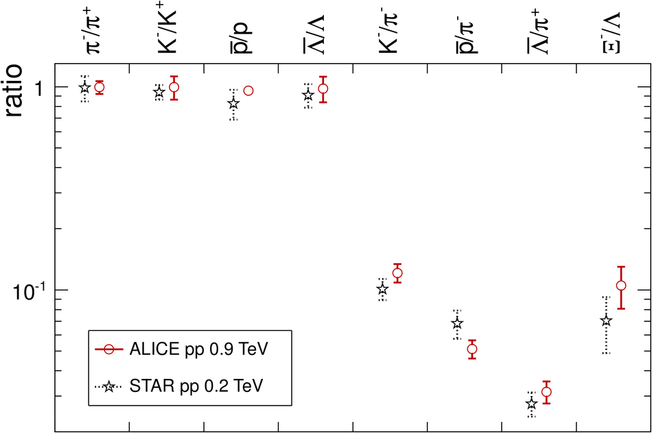 |
Figure 20
< $p_{\mathrm{T}}$> vs. particle mass for the measurements performed with the ALICE experiment and compared with STAR values for pp collisions at $\sqrt{s}$ = 0.2 $\tev$ [25,28] and the ISR parameterization [29]. Both statistical (vertical error bars) and systematic (brackets) uncertainties are shown for ALICE data | 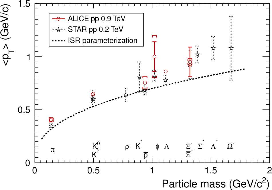 |
Figure 21
($\mathrm {\Lambda}$+$\mathrm {\overline{\Lambda}}$)/2$\Kzs$ as a function of $\pT$ for different collision energiesin pp and $\ppbar$ minimum bias events The STAR ratio is taken from whereas the CDF and UA1 ratios are computed with the ($\mathrm {\Lambda}$+$\mathrm {\overline{\Lambda}}$) and $\Kzs$ spectra published in and respectively The ALICE and STAR ratios are feed-down corrected Because the $\Kzs$ and ($\mathrm {\Lambda}$+$\mathrm {\overline{\Lambda}}$) spectra from UA1 have incompatible binning, the $\Kzs$ differential yield has been calculated for each ($\mathrm {\Lambda}$+$\mathrm {\overline{\Lambda}}$) $\pT$ data point using the fit function published by UA1. Such a choice is motivated by the fact that the $\chi^{2}$ value for the $\Kzs$ spectrum fit is better than that for the ($\mathrm {\Lambda}$+$\mathrm {\overline{\Lambda}}$) spectrum. | 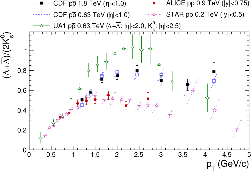 |