Measurements of the $p_{\rm T}$-dependent flow vector fluctuations in Pb-Pb collisions at $\sqrt{s_{_{\rm NN}}} = 5.02~\mathrm{TeV}$ using azimuthal correlations with the ALICE experiment at the Large Hadron Collider are presented. A four-particle correlation approach [1] is used to quantify the effects of flow angle and magnitude fluctuations separately. This paper extends previous studies to additional centrality intervals and provides measurements of the $p_{\rm T}$-dependent flow vector fluctuations at $\sqrt{s_{_{\rm NN}}} = 5.02~\mathrm{TeV}$ with two-particle correlations. Significant $p_{\rm T}$-dependent fluctuations of the $\vec{V}_{2}$ flow vector in Pb-Pb collisions are found across different centrality ranges, with the largest fluctuations of up to $\sim$15% being present in the 5% most central collisions. In parallel, no evidence of significant $p_{\rm T}$-dependent fluctuations of $\vec{V}_{3}$ or $\vec{V}_{4}$ is found. Additionally, evidence of flow angle and magnitude fluctuations is observed with more than $5\sigma$ significance in central collisions. These observations in Pb-Pb collisions indicate where the classical picture of hydrodynamic modeling with a common symmetry plane breaks down. This has implications for hard probes at high $p_{\rm T}$, which might be biased by $p_{\rm T}$-dependent flow angle fluctuations of at least 23% in central collisions. Given the presented results, existing theoretical models should be re-examined to improve our understanding of initial conditions, quark--gluon plasma properties, and the dynamic evolution of the created system.
Phys. Rev. C 109 (2024) 065202
HEP Data
e-Print: arXiv:2403.15213 | PDF | inSPIRE
CERN-EP-2024-084
Figure group
Figure 1
The ratio $v_2\{2\}/v_2[2]$ in Pb-Pb collisions at $\snn$ = 5.02 TeV (solid dark blue circles) and 2.76 TeV (open light blue circles) as a function of transverse momentum. The different panels display results in different centrality intervals. Statistical (systematic) uncertainties are represented by solid bars (faded boxes). Predictions from the iEBE-VISHNU hydrodynamic model with T$_{\rm R}$ENTo initial conditions and temperature-dependent $\eta/s(T)$ , and with AMPT initial conditions and $\eta/s = 0.08$ , are shown in colored bands. | 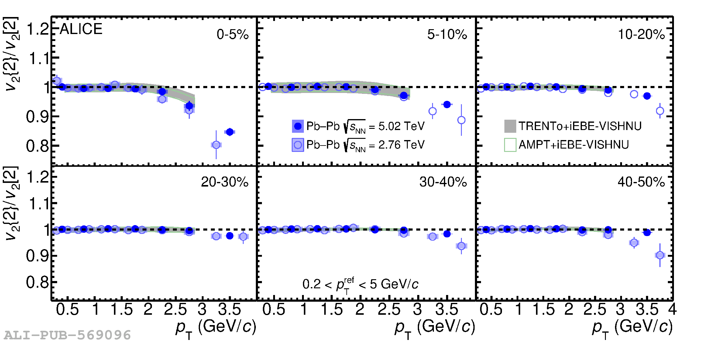 |
Figure 2
The ratio $v_3\{2\}/v_3[2]$ for Pb-Pb collisions at $\snn$ = 5.02 TeV (solid dark red squares) and 2.76 TeV (open light red squares) as a function of transverse momentum. The different panels display results in different centrality intervals. Statistical (systematic) uncertainties are represented by solid bars (faded boxes). Predictions from iEBE-VISHNU hydrodynamic model with T$_{\rm R}$ENTo initial conditions and temperature-dependent $\eta/s(T)$ , and with AMPT initial conditions and $\eta/s = 0.08$ , are shown in colored bands. | 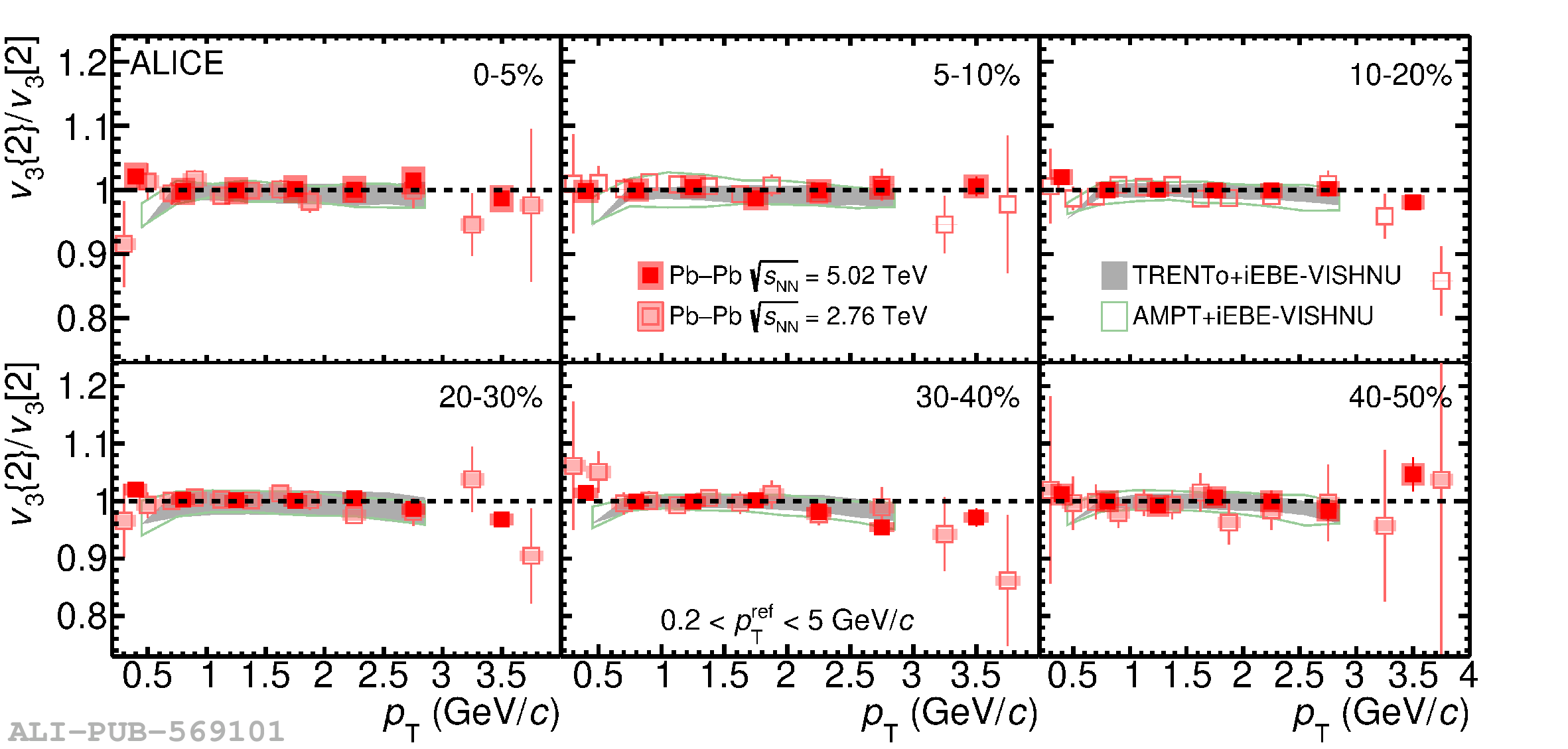 |
Figure 3
The ratio $v_4\{2\}/v_4[2]$ for Pb-Pb collisions at $\snn$ = 5.02 TeV (solid dark cyan triangles) and 2.76 TeV (open light cyan triangles) as a function of transverse momentum. The different panels display results in different centrality intervals. Statistical (systematic) uncertainties are represented by solid bars (faded boxes). Comparison with iEBE-VISHNU hydrodynamic model with T$_{\rm R}$ENTo initial conditions and temperature-dependent $\eta/s(T)$ , and with AMPT initial conditions and $\eta/s = 0.08$ , are shown in colored bands. | 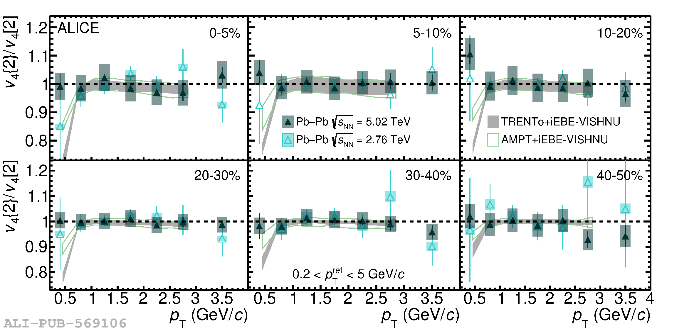 |
Figure 4
The factorization ratio $r_2$ for Pb-Pb collisions at $\snn$ = 5.02 TeV (dark blue circles) and 2.76 TeV (light blue circles) as a function of associated particle $p_{\rm T}^{\rm a}$. The columns show the results in centrality intervals 0--5\%, 20--30\%, and 40--50\%, while the rows show the results for different trigger particle $p_\mathrm{T}^t$ intervals. Statistical (systematic) uncertainties are represented by solid bars (faded boxes). | 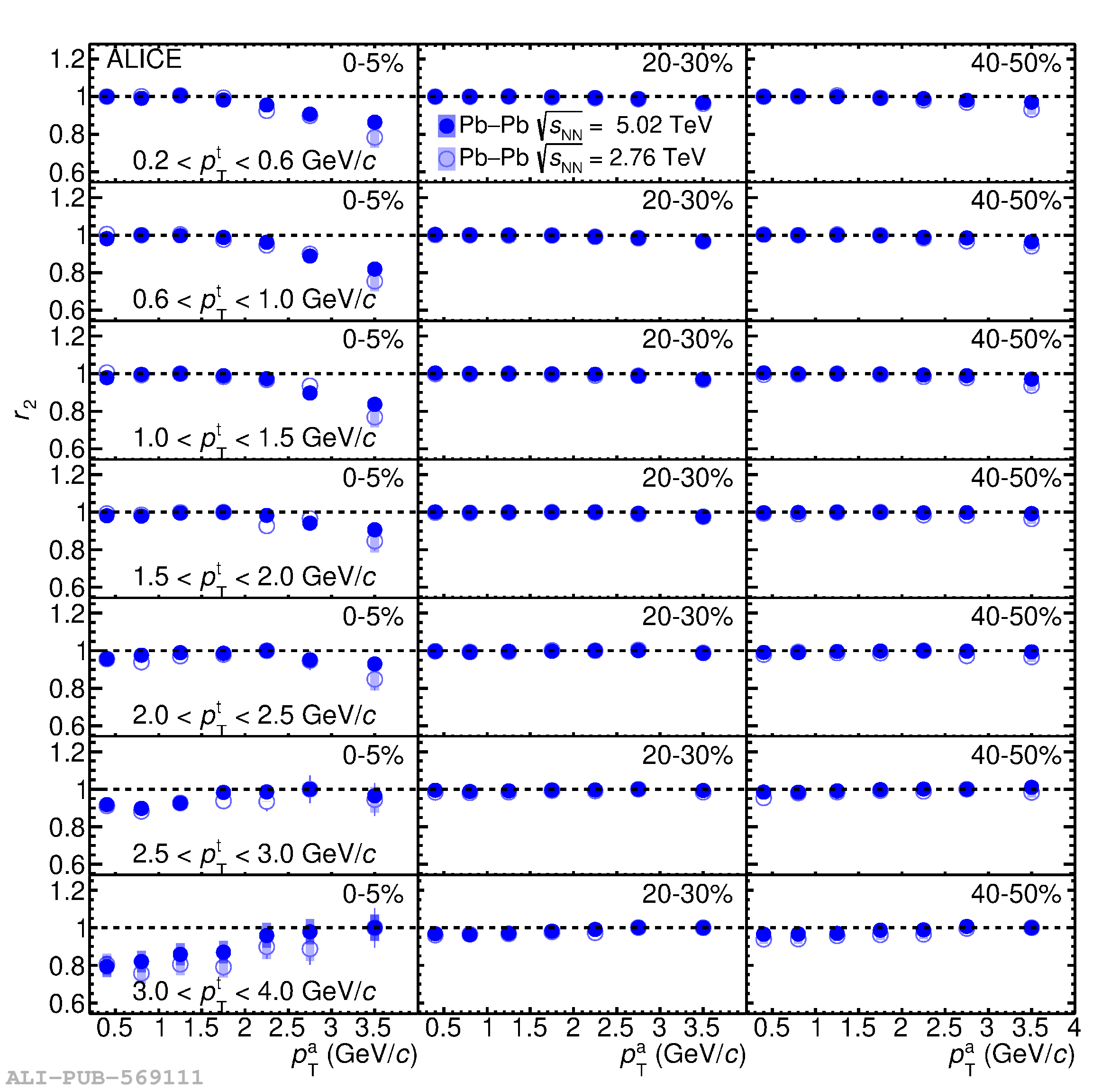 |
Figure 5
The factorization ratio $r_2$ for Pb-Pb collisions at $\snn$ = 5.02 TeV (blue circles) as a function of $p_{\rm T}^{\rm a}$ for $0.2 < p_{\rm T}^{\rm t} < 0.6$ GeV/c. The different panels display results in different centrality intervals. Statistical (systematic) uncertainties are represented by solid bars (faded boxes). Predictions from iEBE-VISHNU hydrodynamic model with T$_{\rm R}$ENTo initial conditions and temperature-dependent $\eta/s(T)$ , and with AMPT initial conditions and $\eta/s = 0.08$ , are shown in colored bands. | 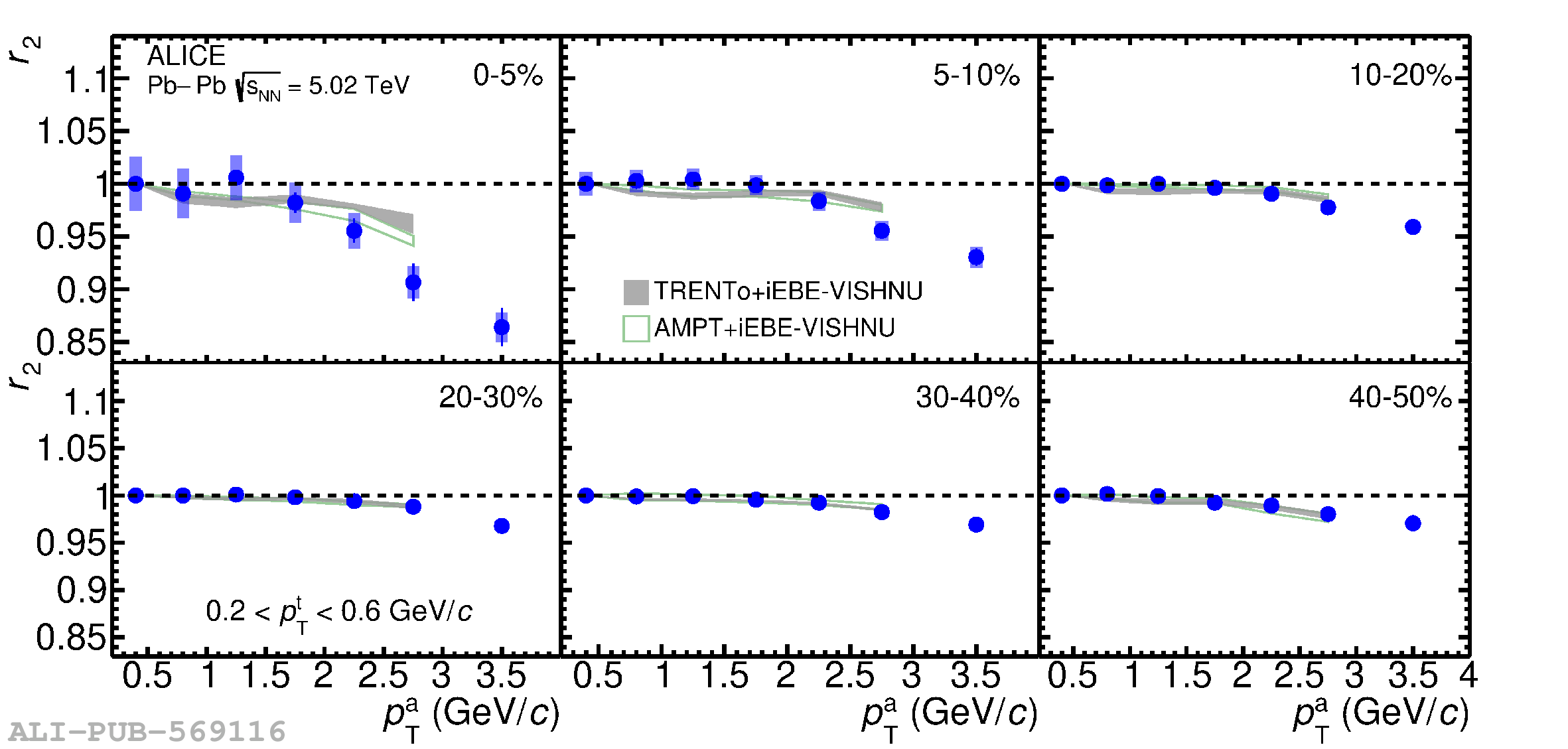 |
Figure 6
The factorization ratio $r_3$ in Pb-Pb collisions at $\snn$ = 5.02 TeV (solid dark red squares) and 2.76 TeV (open light red squares) as a function of $p_{\rm T}^{\rm a}$. The columns show the results in centrality intervals 0--5\%, 20--30\%, and 40--50\%, while the rows show the results for different trigger particle $p_\mathrm{T}^t$ intervals. Statistical (systematic) uncertainties are represented by solid bars (faded boxes). | 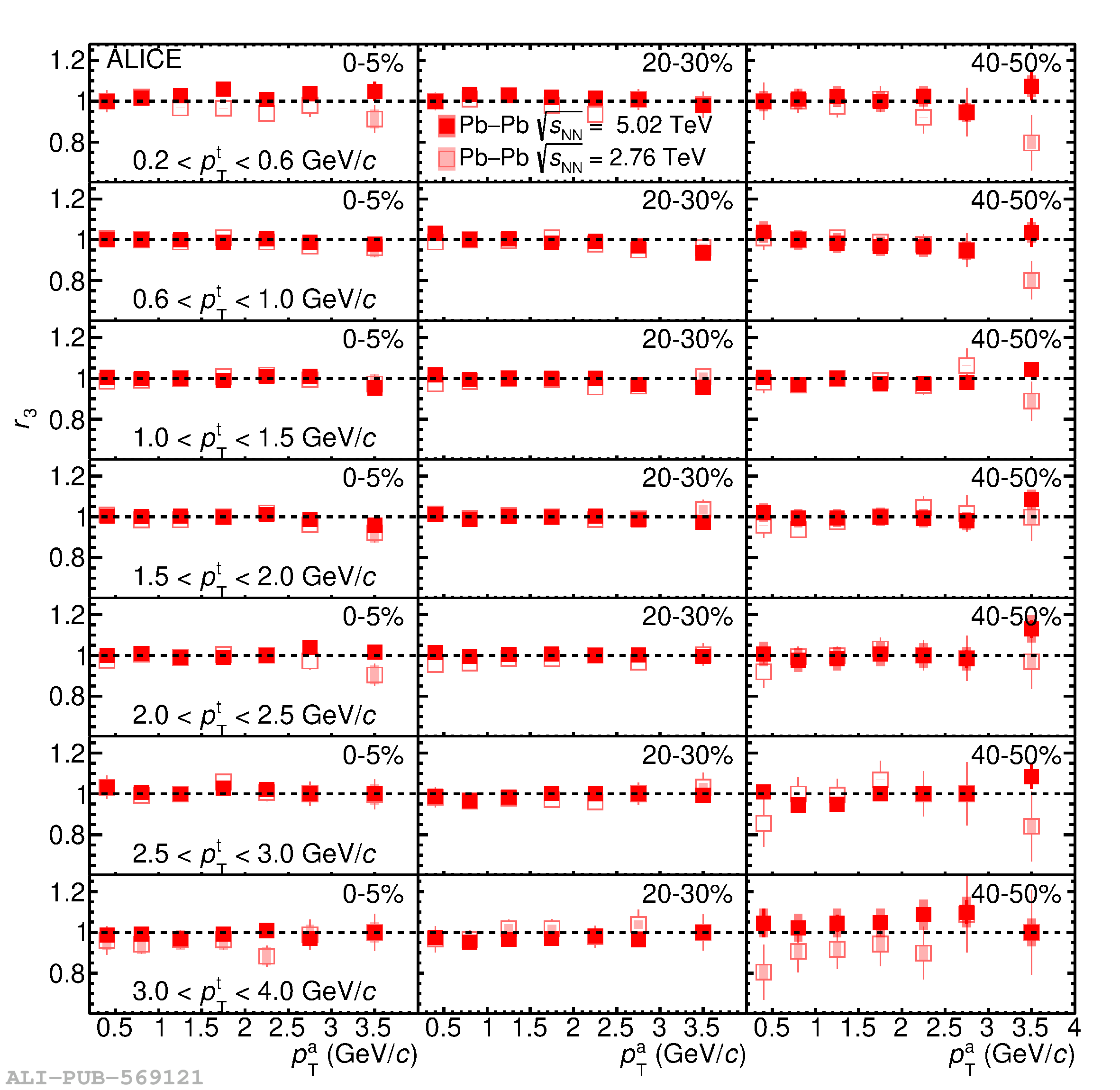 |
Figure 7
The flow angle fluctuations $A_2^{\rm f}$ in Pb-Pb collisions at $\snn$ = 5.02 TeV (blue circles) as a function of $\pt$. The different panels display results in different centrality intervals. Statistical (systematic) uncertainties are represented by solid bars (faded boxes). Predictions from iEBE-VISHNU with AMPT initial conditions and $\eta/s = 0.08, 0.20$ and iEBE-VISHNU with \trento initial conditions and $\eta/s(T)$ as well as AMPT are shown in colored bands. | 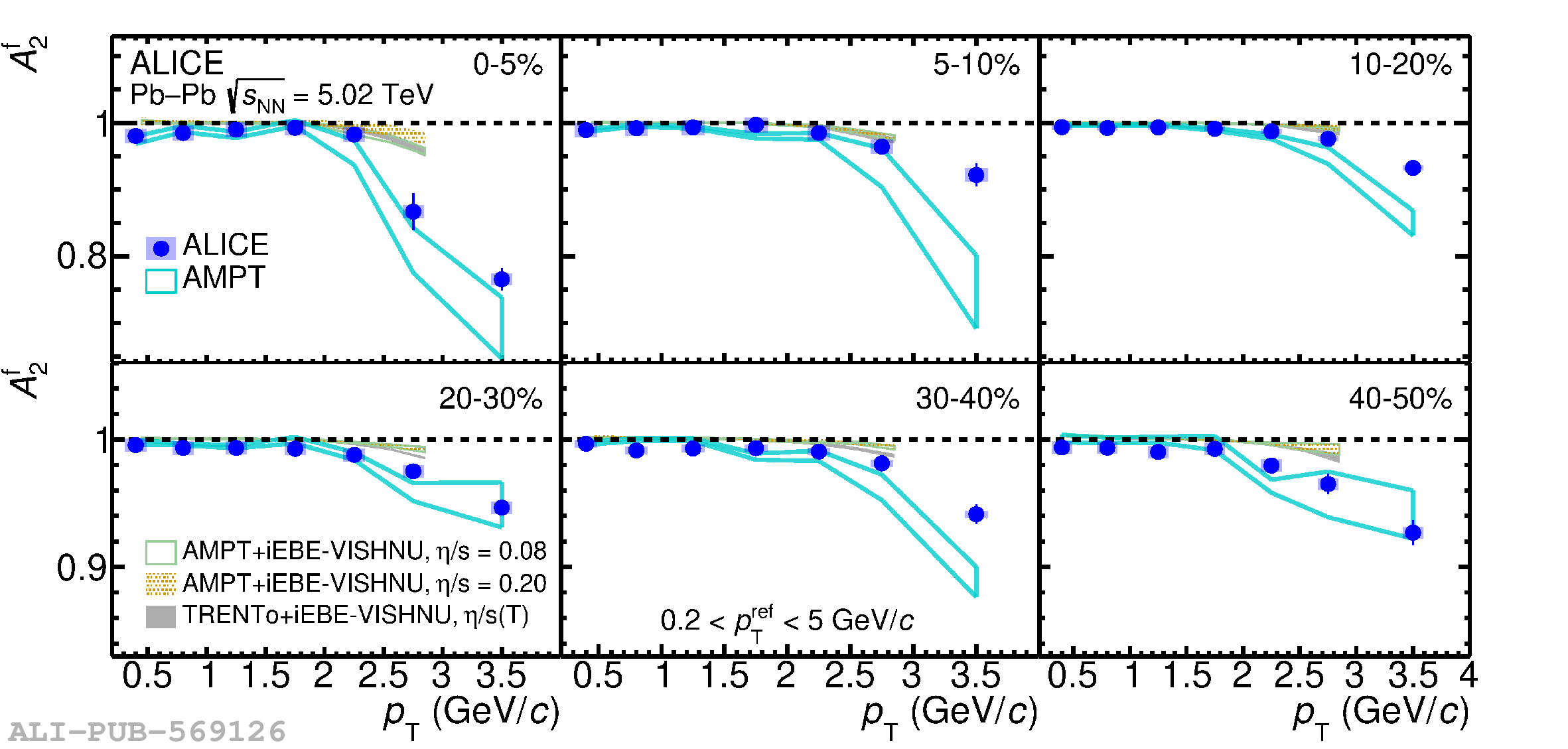 |
Figure 8
The flow magnitude fluctuations $M_2^{\rm f}$ in Pb-Pb collisions at $\snn$ = 5.02 TeV (red squares) as a function of $\pt$. The different panels display results in different centrality intervals. Statistical (systematic) uncertainties are represented by solid bars (faded boxes). Predictions from iEBE-VISHNU with AMPT initial conditions and $\eta/s = 0.08, 0.20$ and iEBE-VISHNU with \trento initial conditions and $\eta/s(T)$ as well as AMPT are shown in colored bands. | 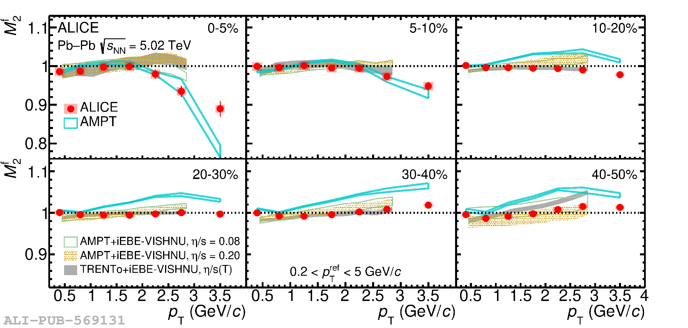 |
Figure 9
The lower limit of $\langle \cos n(\Psi_2(\pt)-\Psi_2)\rangle$ (blue boxes), the upper limit of $\langle v_2(\pt)v_2\rangle/\sqrt{\langle v_2^2(\pt)\rangle\langle v_2^2\rangle}$ (red boxes), and the flow vector fluctuations $v_{2}\{2\}/v_2[2]$ (gray diamonds) as a function of $\pt$. The different panels display results in different centrality intervals. The red (blue) arrows denote the upper (lower) limits, and the statistical (systematic) uncertainties are represented by open (shaded) boxes. | 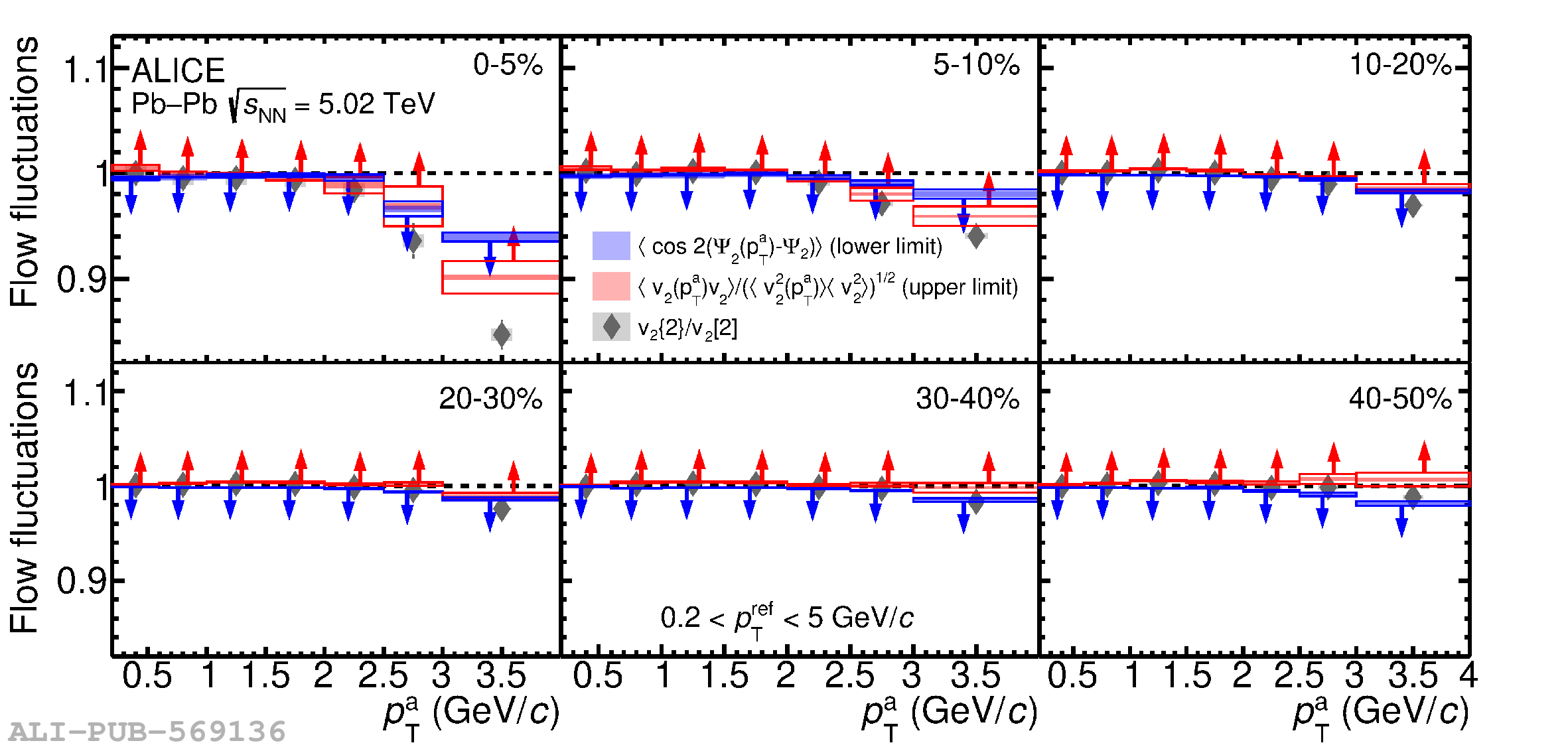 |