The procedure for the energy calibration of the high granularity electromagnetic calorimeter PHOS of the ALICE experiment is presented. The methods used to perform the relative gain calibration, to evaluate the geometrical alignment and the corresponding correction of the absolute energy scale, to obtain the nonlinearity correction coefficients and finally, to calculate the time-dependent calibration corrections, are discussed and illustrated by the PHOS performance in proton-proton (pp) collisions at $\sqrt{s}$ = 13 TeV. After applying all corrections, the achieved mass resolutions for $\pi^0$ and $\eta$ mesons for $p_{\rm{T}} > 1.7$ GeV/$c$ are $\sigma_m^{\pi^0} = 4.56 \pm 0.03$ MeV/$c^2$ and $\sigma_m^{\eta} = 15.3 \pm 1.0$ MeV/$c^2$, respectively.
JINST 14 (2019) 05, P05025
e-Print: arXiv:1902.06145 | PDF | inSPIRE
CERN-EP-2019-020
Figure 1
[Color online] ALICE cross-sectional view in Run 2, PHOS modules are located at the bottom of the setup. | 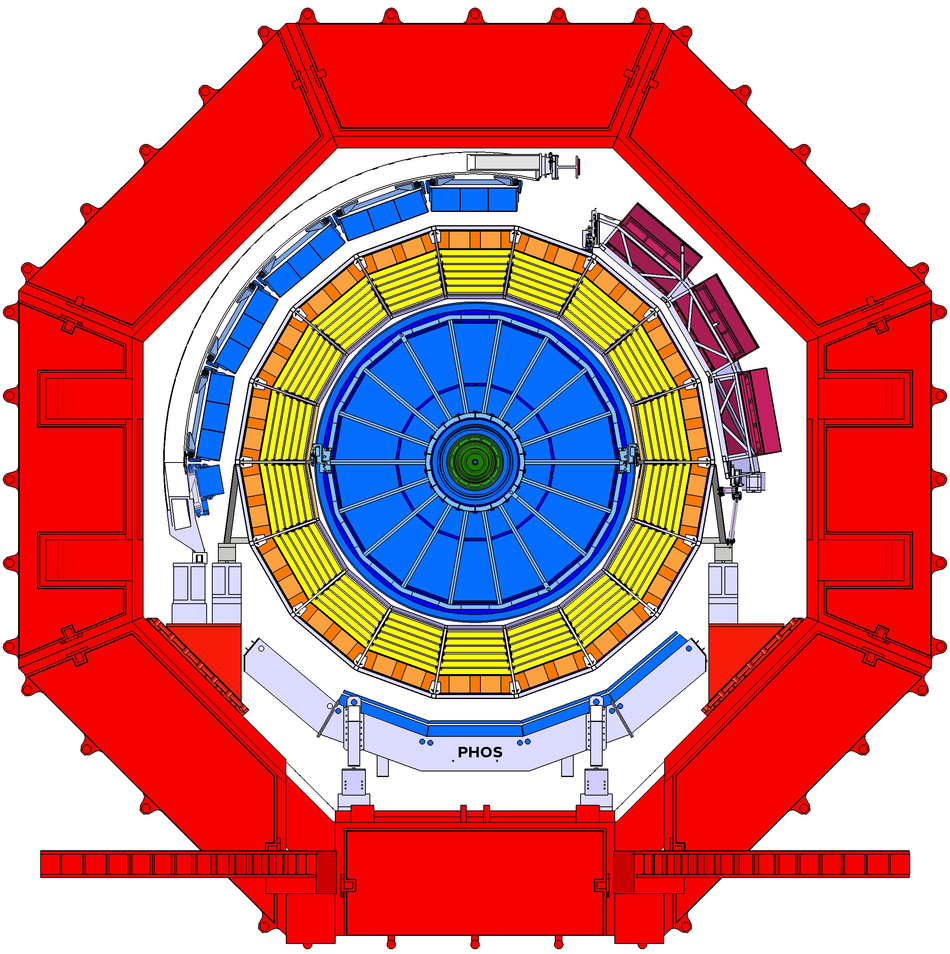 |

Figure 6
[Color online] Invariant mass distribution of cluster pairs after APD gain equalization in pp collisions at $\sqrt{s}=13$ TeV for $\pT>1.7 \GeVc$. The red curve is a fit of the spectrum with the sum of a Gaussian and a second-order polynomial function. The green dashed line is the background contribution only. | 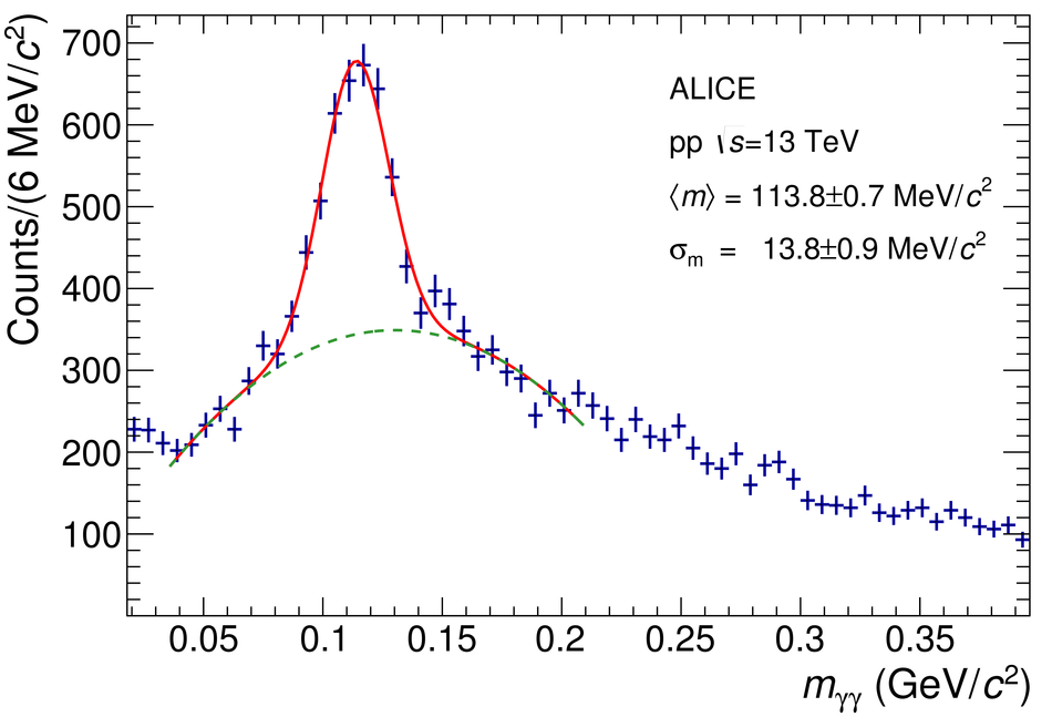 |
Figure 7
[Color online]Study using a toy Monte Carlo simulation of the convergence of the iterative calibration procedure based on equalization of the $\pi^0$ peak position. The residual de-calibration $\sigma_{\rm c}$ is shown as a function of the iteration number. Two values of calorimeter energy resolution are considered, standard ($\sigma_{E}$) and twice as poor ($2\sigma_{E}$). | 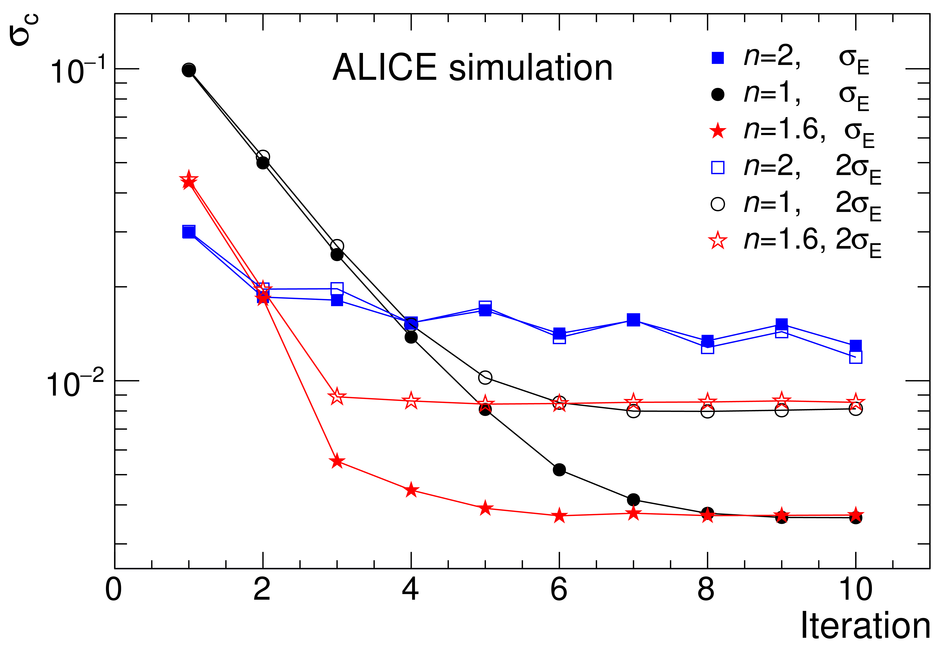 |
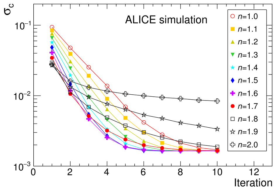
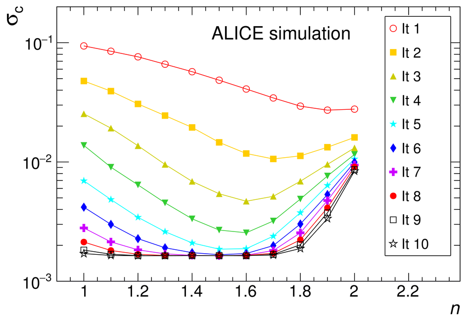

Figure 13
[Color online] Dependence of the mean distance between track extrapolation to the PHOS surface and cluster position in the cluster coordinate on the PHOS plane along (left) and perpendicular(right), to the beam and magnetic field direction. In the left plot contributions of electrons and positrons are combined. The dependencies are fitted with linear functions and the resulting slopes are shown in both legends. | 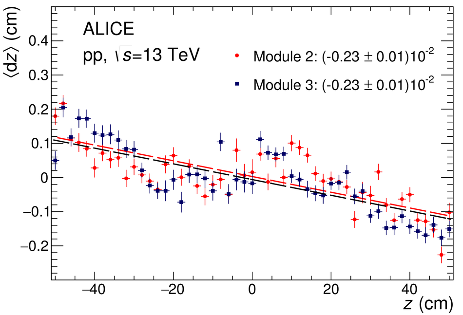 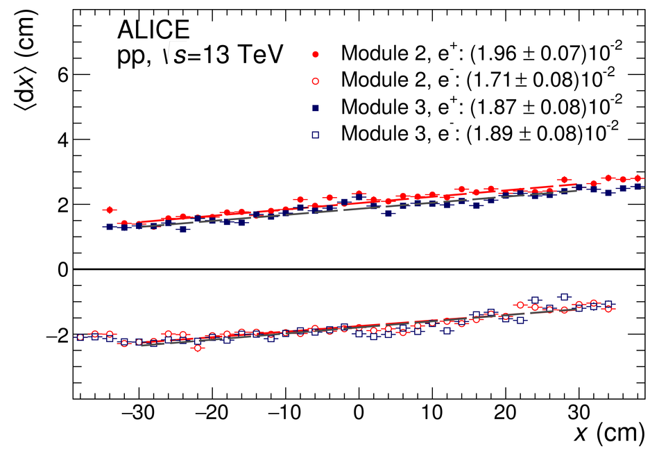 |
Figure 15
[Color online] Left: the $\pi^0$ peak position as a function of the transverse momentum for several values of nonlinearity parameters ($d$, $e$), with default values for $a$, $b$ and $c$. Right: the deviation from a constant value of the $\pi^0$ peak position expressed in $\chi^2/NDF$ as a function of the nonlinearity parameters ($d$, $e$). | 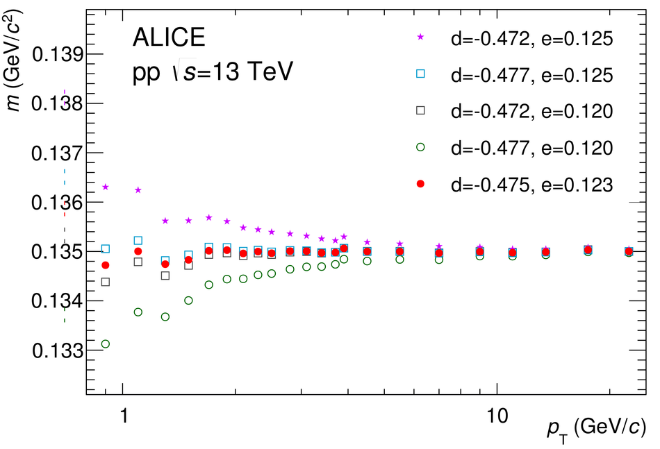 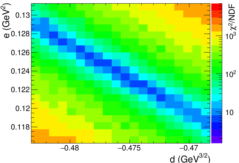 |
Figure 17
[Color online] Invariant mass distributions of cluster pairs for $\pT>1.7 \GeVc$ in the $\pi^0$ (left) and $\eta$ (right) mass region after calibration with per-channel $\pi^0$ peak equalization. For the $\pi^0$ data, the solid curve shows the fitting function using thesum of the Crystal Ball and a polynomial function. For the $\eta$ data, the solid curve shows the fit function composed of a Gaussian and a polynomial function. The dashed lines represent the background contributions in both plots. | 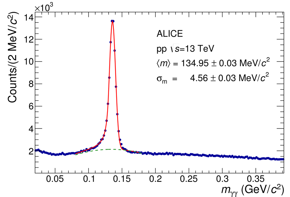 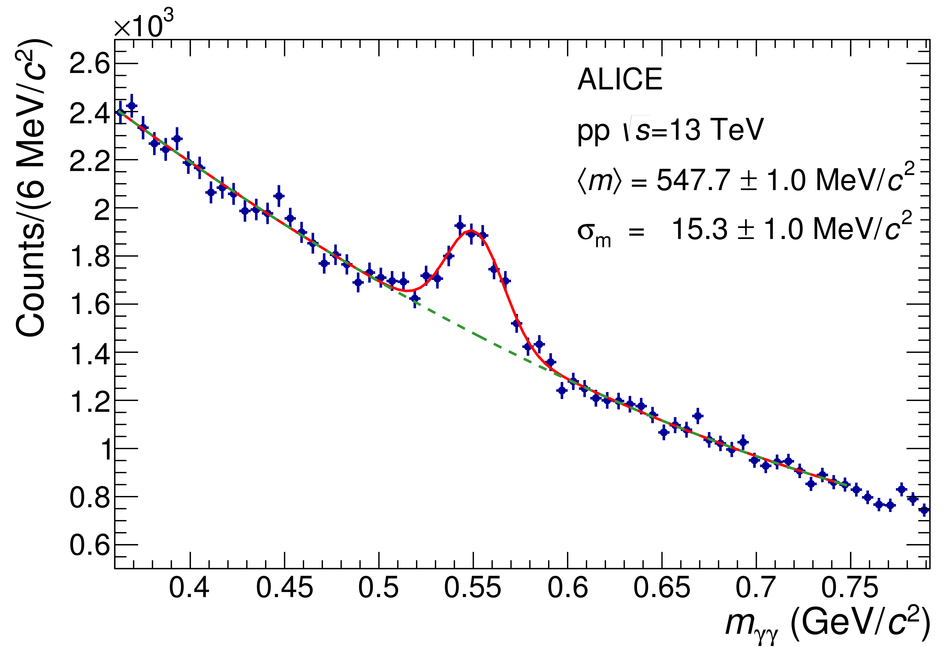 |