Global fit examples in $0$--$10$% central events for $n=2,3,4$ and $5$. The measured ${V_{n\Delta}}$ coefficients are plotted on an interleaved ${p_{T}^{t}}$, ${p_{T}^{a}}$ axis in the upper panels, and the global fit function (Eq. 6}) is shown as the red curves. The global fit systematic uncertainty is represented by dashed lines. The lower section of each panel shows the ratio of the data to the fit, and the shaded bands represent the systematic uncertainty propagated to the ratio. In all cases, off-scale points are indicated with arrows.
\begin{align*} (6)   V_{n\Delta} ({p_{T}^{t}}, {p_{T}^{a}}) &=& \langle\langle e^{in(\phi_a - \phi_t)} \rangle \rangle \nonumber \\ &=& \langle \langle e^{in(\phi_a - \Psi_n)} \rangle \langle e^{-in(\phi_t - \Psi_n)} \rangle \rangle \nonumber \\ &=& \langle v_n\{2\}({p_{T}^{t}}) \, v_n\{2\}({p_{T}^{a}}) \rangle \end{align*}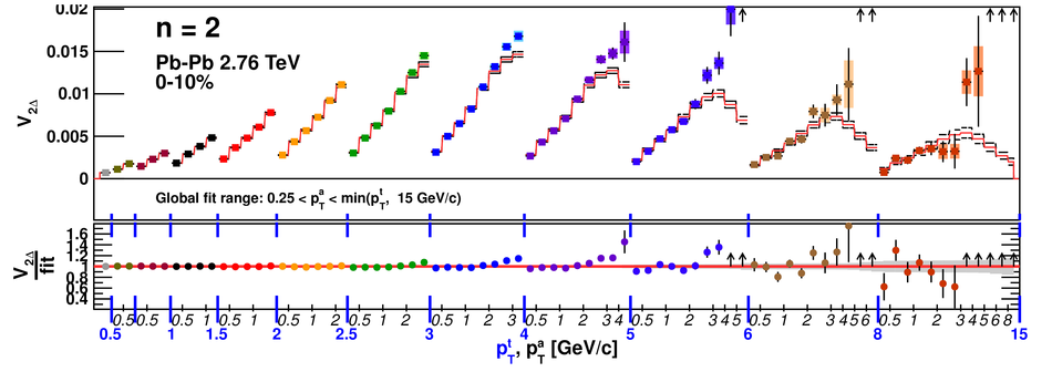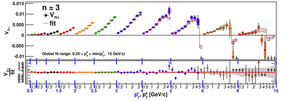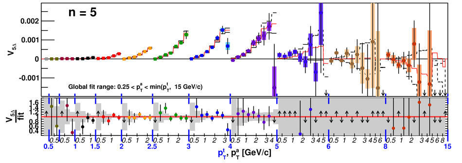