Femtoscopic analysis can shed light on hadron production in pp collisions. In this paper, proton-proton correlations measured in collisions at $\sqrt{s}=13.6$ TeV recorded with the ALICE detector at the LHC are presented. The analysis is based on the minimum bias dataset collected in 2022 following the upgrade of the ALICE detector and corresponds to an integrated luminosity of $19.3$ pb$^{-1}$. The increased integrated luminosity allows us, for the first time, to simultaneously measure the multiplicity and transverse-mass ($m_{\rm T}$) dependence of the size of the hadron-emitting source. Precise knowledge of the femtoscopic source size in pp collisions is a crucial ingredient for using femtoscopy to study the residual strong interaction among stable and unstable hadrons at the LHC. In this light, the source radius was determined from the measured correlation functions by assuming several state-of-the-art models of the nucleon$-$nucleon interactions. The consistency among the extracted radii demonstrates the robustness of the measurement with respect to interaction model assumptions. A comparison to femtoscopic radii measured in Pb$-$Pb collisions at $\sqrt{s}=5.02$ TeV reveals a markedly different multiplicity dependence in similar $m_{\rm T}$ intervals, providing new insight into the system-size dependence of particle emission dynamics.
Submitted to: EPJC
e-Print: arXiv:2606.28098 | PDF | inSPIRE
CERN-EP-2026-180
Figure group
Figure 2
Left panel: the real part of the \pP wave functions obtained from the four variations of the Norfolk potential (black and blue lines together with black axis) and the two Gaussian source distributions (red lines with red axis) as a function of the relative nucleon--nucleon distance $r$. Right panel: the calculated \pP correlation functions for all the potential variations and the two source radii. The correlation functions for the four variations of the Norfolk potential are indistinguishable. See text for details. | 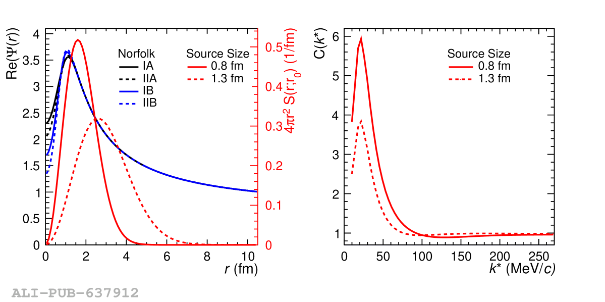 |
Figure 3
Fits of the measured \pP (upper row) and \ApAp (lower row) correlation functions in all multiplicity ranges and \mT range $[1.02, 1.14]\, \si{\gevcc}$ fitted with the RSM. The total fit with uncertainties is indicated by the blue band and the baseline with uncertainties is indicated by the red band. Statistical uncertainties are indicated by the vertical error bars and are smaller than the markers. Systematic uncertainties are indicated by the gray shaded boxes. The markers are positioned in each \kstar bin at the mean value of the underlying \kstar distribution and the horizontal lines indicate the standard deviation of the \kstar distribution within the bin. The deviation of the data points to the total fit in terms of standard deviations is shown in the lower panel. | 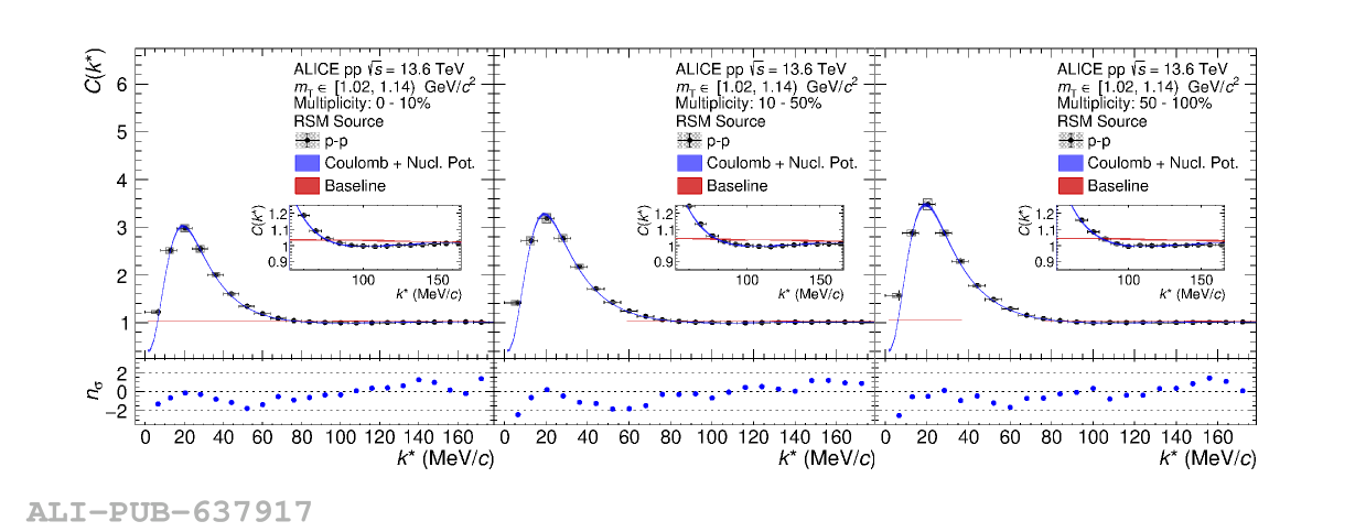 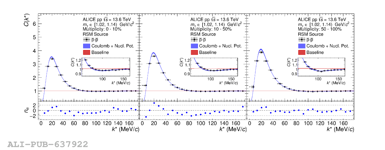 |
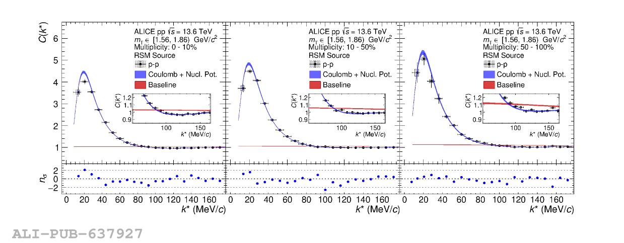
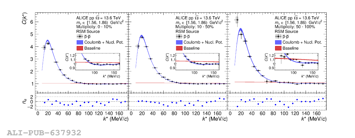
Figure 5
The \mT dependence of the effective radius \reff (left) and the core radius \rcore (right) for different multiplicity classes. The black data points are from a previous analysis using a high-multiplicity data set collected by ALICE at \onethree . Here, INEL$>0$ refers to inelastic pp collisions with at least one charged particle in the event within $|\eta| 1.0$ , while 0–0.17\% denotes the highest-multiplicity class, corresponding to the top 0.17\% of events in the charged-particle multiplicity distribution. The bands correspond to the parametrization of the \mT dependence for the different multiplicity classes. | 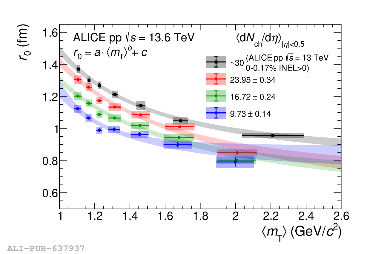 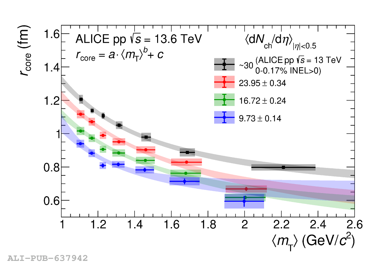 |
Figure 6
The \mT dependence of the effective radius \reff (left) and the core radius \rcore (right) for two different multiplicity classes. The red data points correspond to the extraction of the radii using this analysis's full MB data set. The black data points are from a previous analysis using a high-multiplicity data set collected by ALICE at \onethree . The bands correspond to the parametrization of the \mT dependence for the different multiplicity classes. | 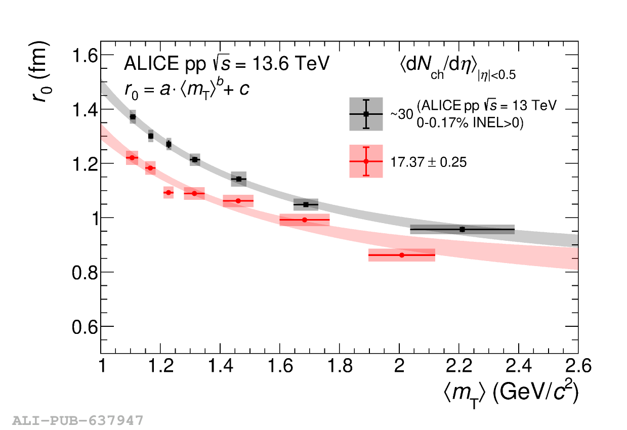 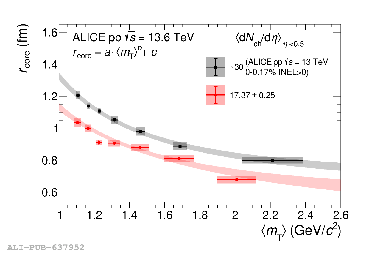 |
Figure 7
Multiplicity dependence of the effective radius \(\reff\) for various \(\mT\) intervals measured in pp and Pb--Pb collisions . The bands represent the parametrization for different multiplicity classes, shown with a \(1\sigma\) uncertainty. Note that the \(\mT\) intervals differ between the two collision systems. | 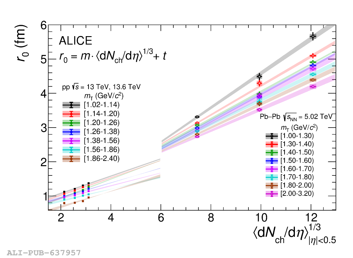 |
Figure A.1
\kstar dependent $\lambda$ parameters for the 0--10\% multiplicity class and the lowest \mT interval (left panel) and the highest \mT interval (right panel). The $\lambda$ parameters for the other \mT intervals can be found on HEPData. The $\lambda$ parameters for protons and antiprotons are shown in a solid and dotted line, respectively. The genuine contributions were scaled down by a factor of 0.6 in order to ensure a better visibility of all lines. | 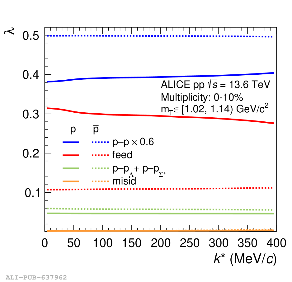 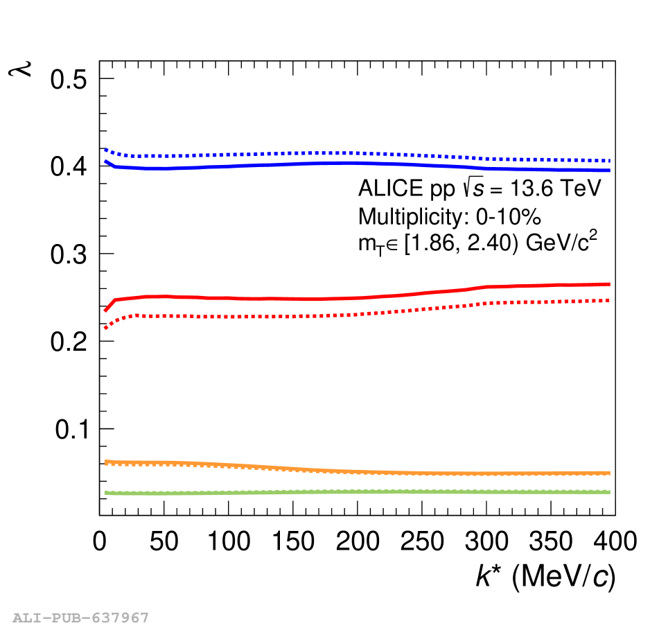 |
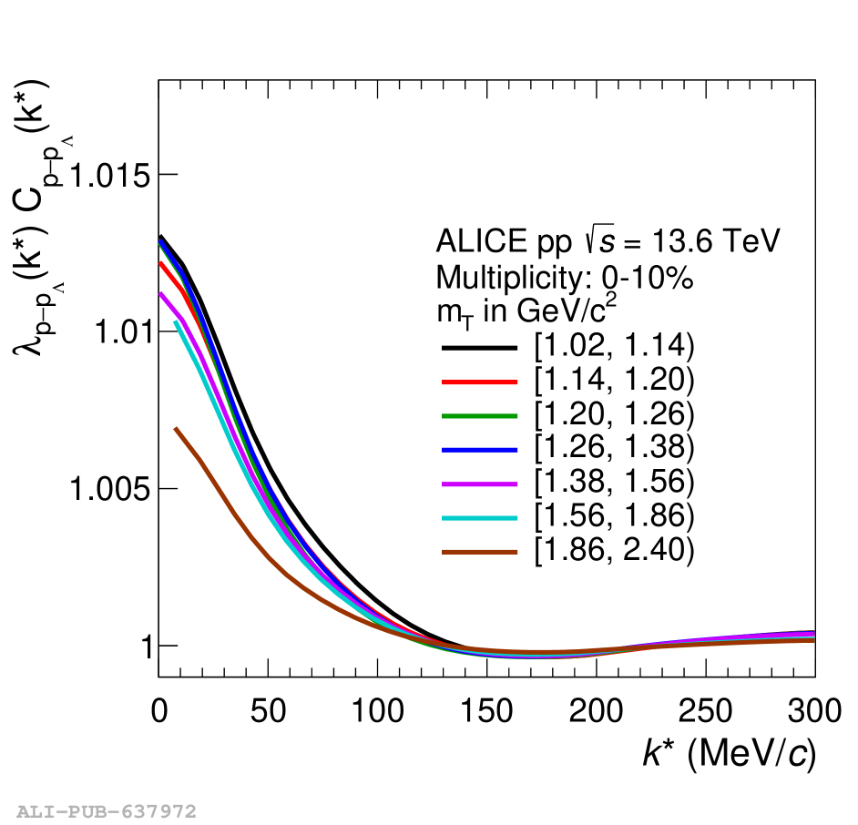
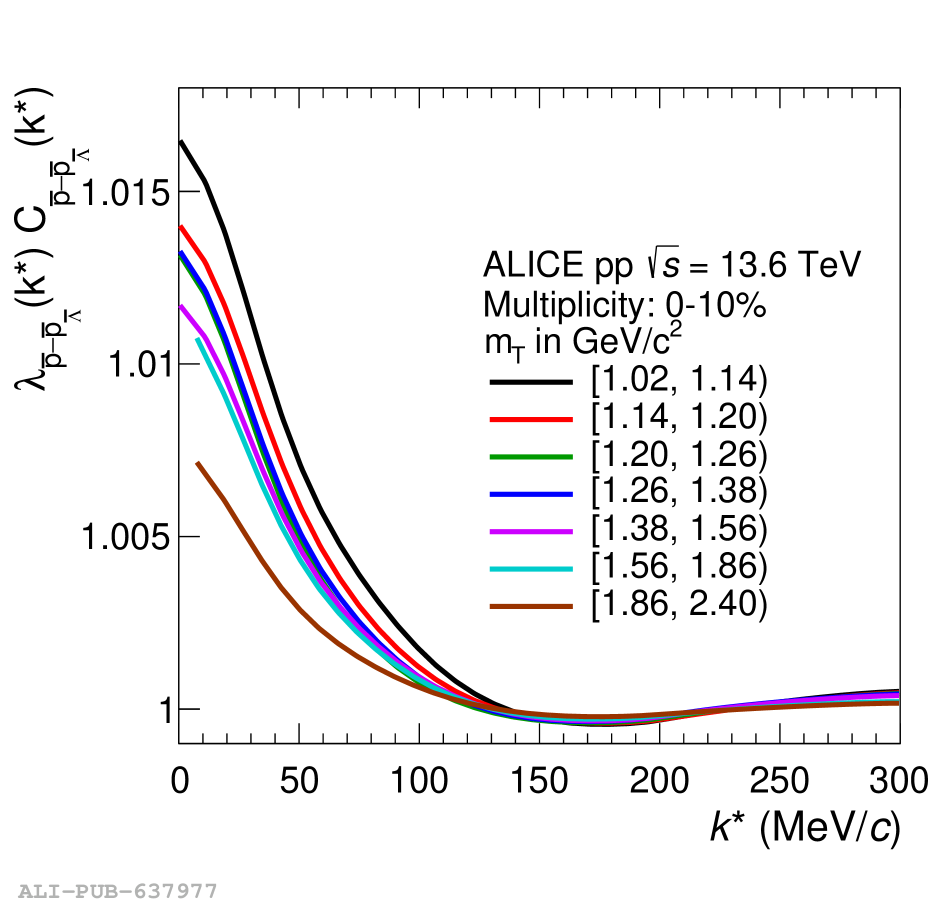
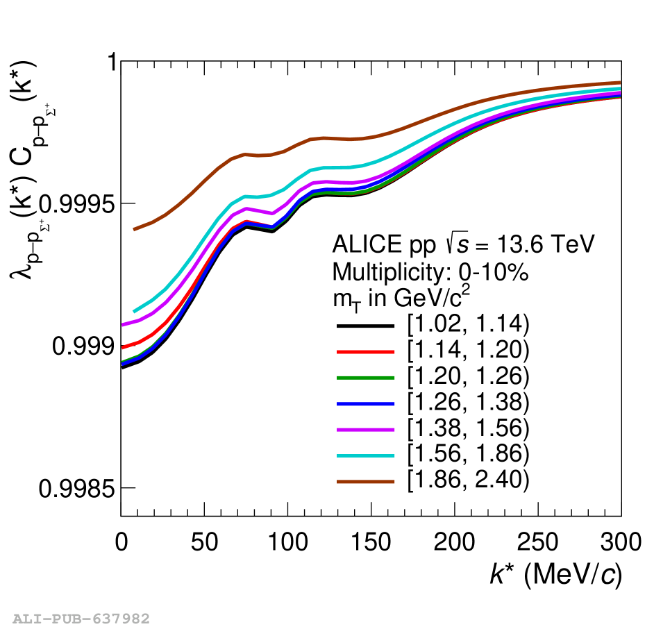
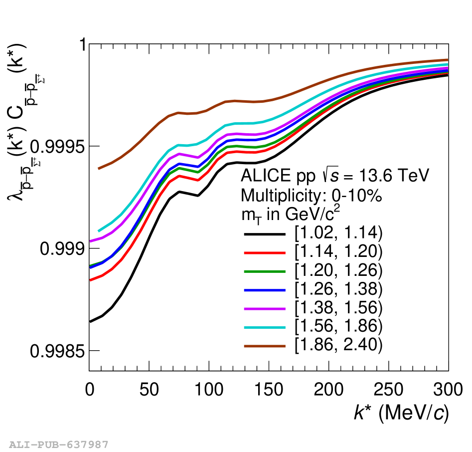
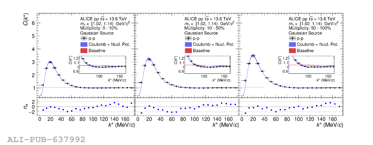
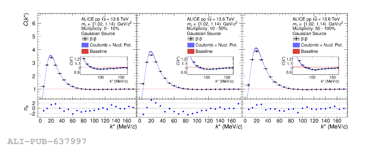

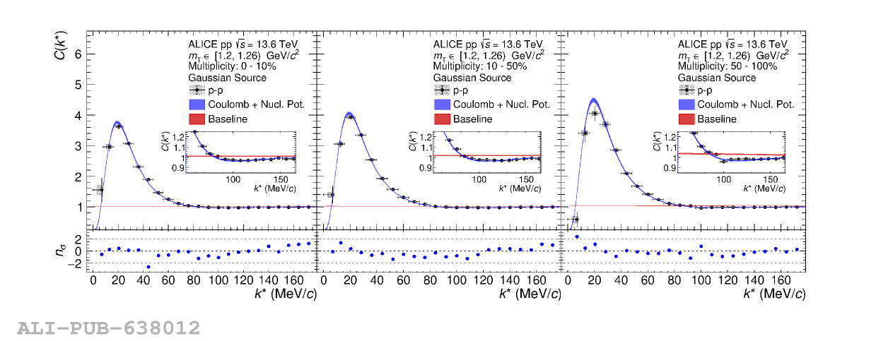

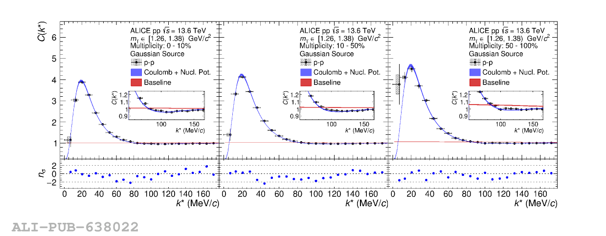
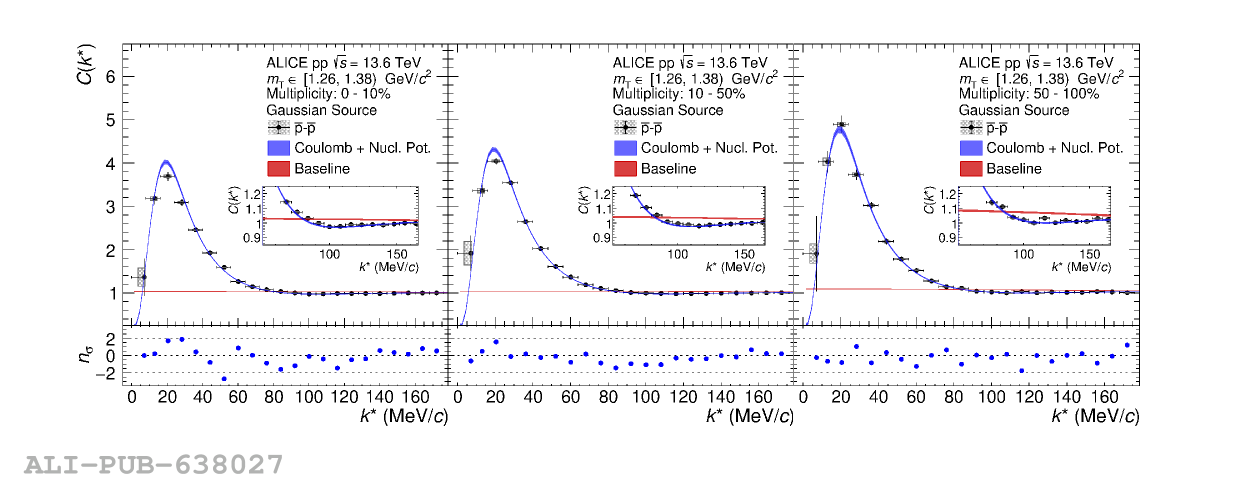
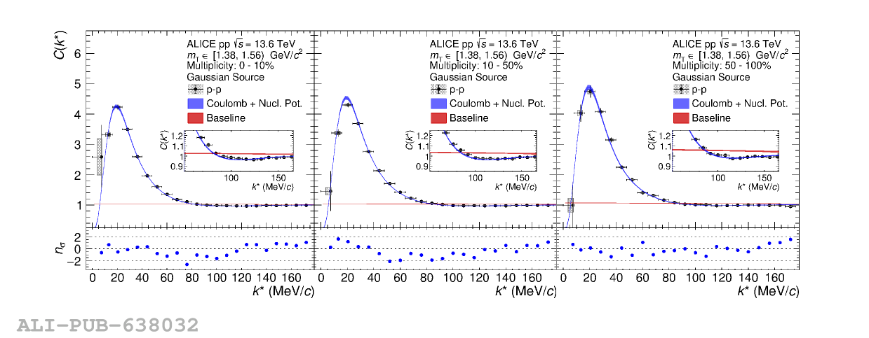

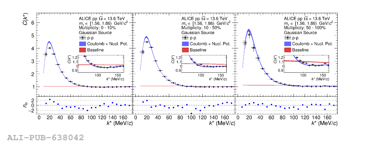
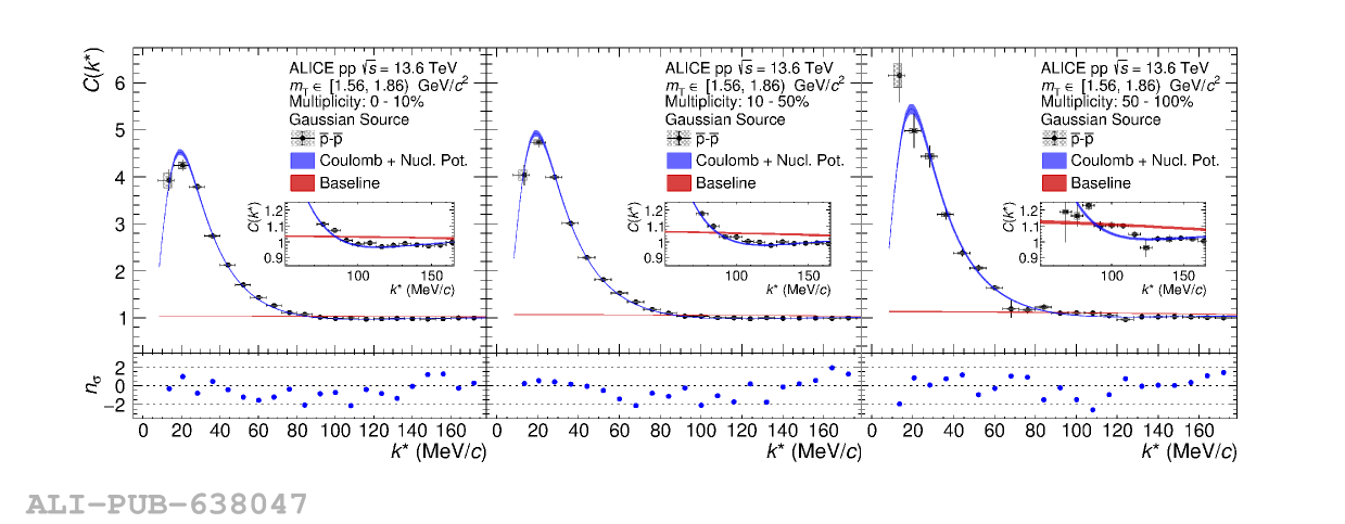
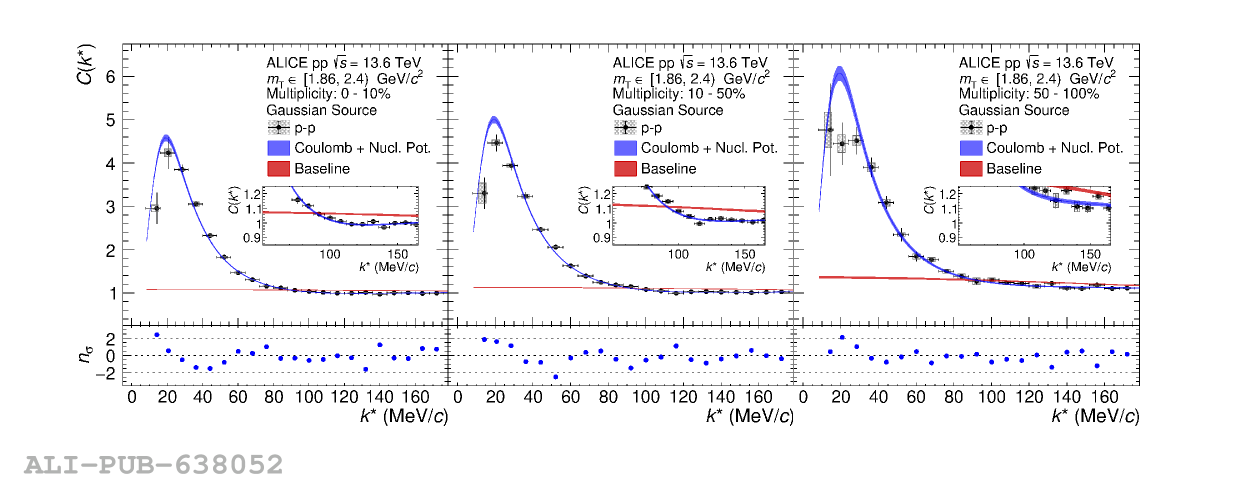
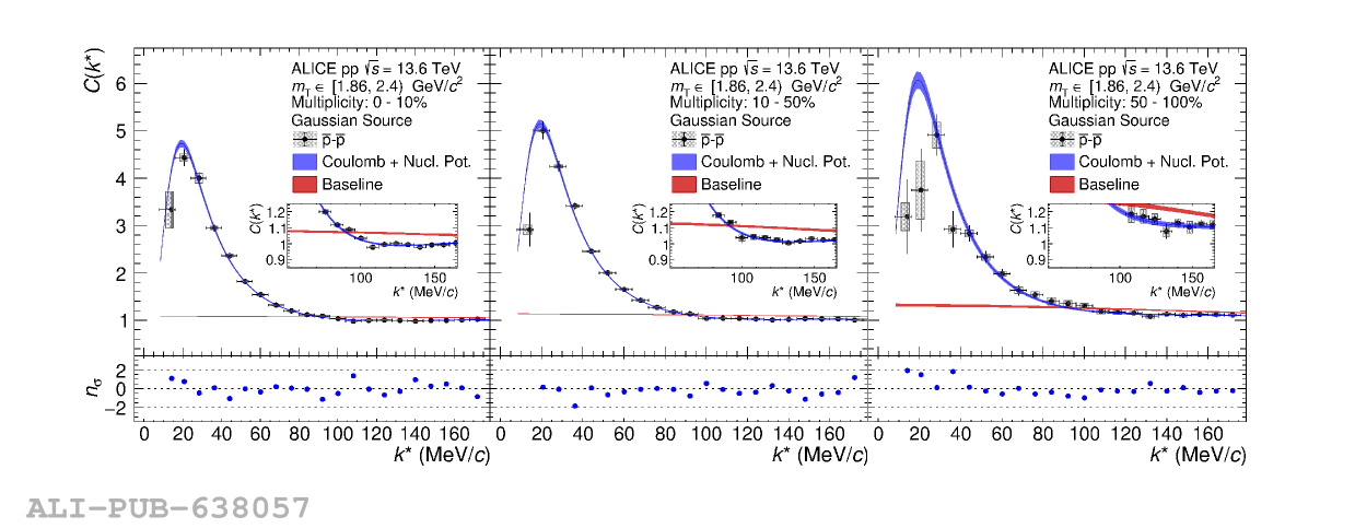
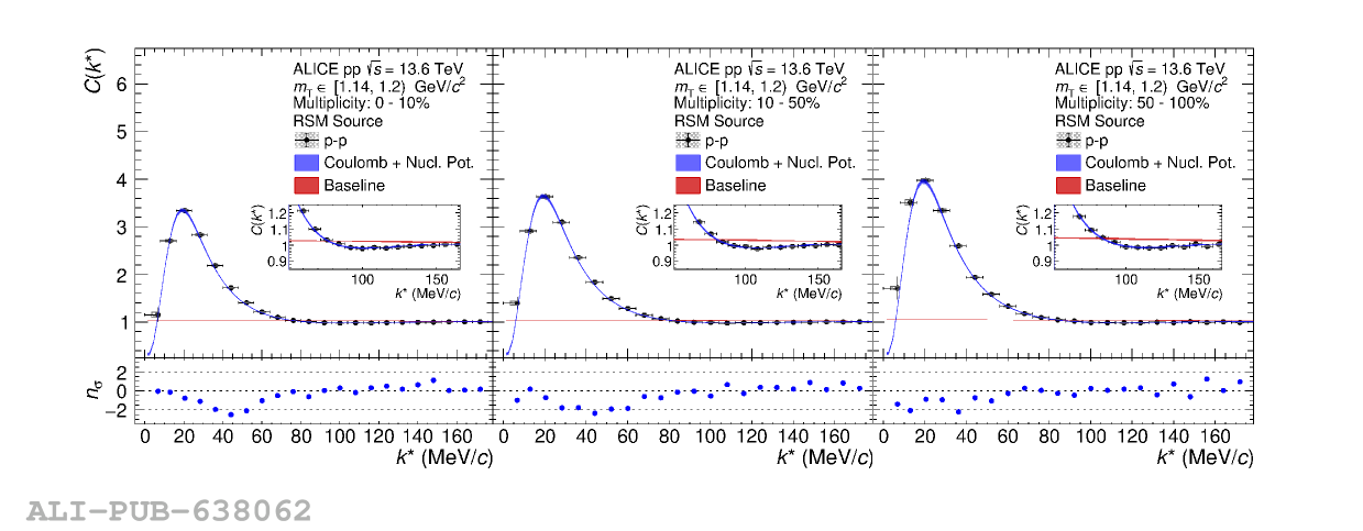
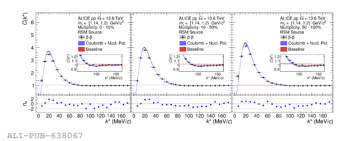
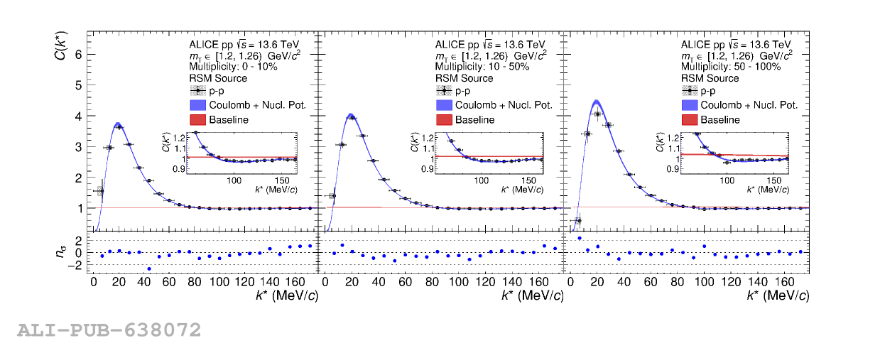
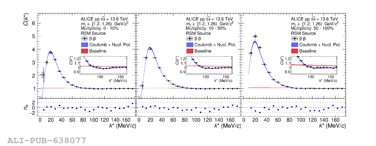
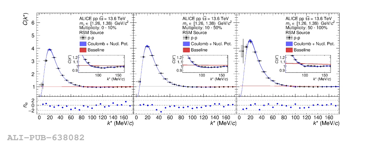
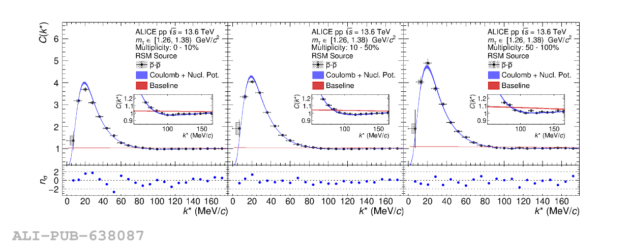
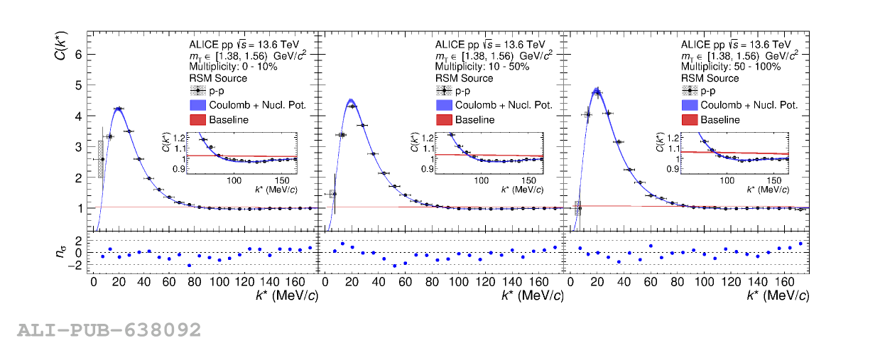
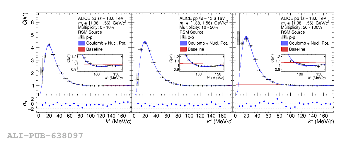
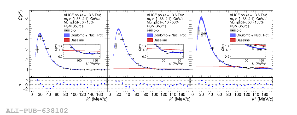

Figure A.16
Fits of the multiplicity integrated \pP (upper row) and \ApAp (lower row) correlation functions using the effective Gaussian source (left column) and the RSM (right column) in the \mT range $[1.02, 1.14]\, \si{\gevcc}$. For a detailed description of the panels see \cref{fig:fitsMt0}. | 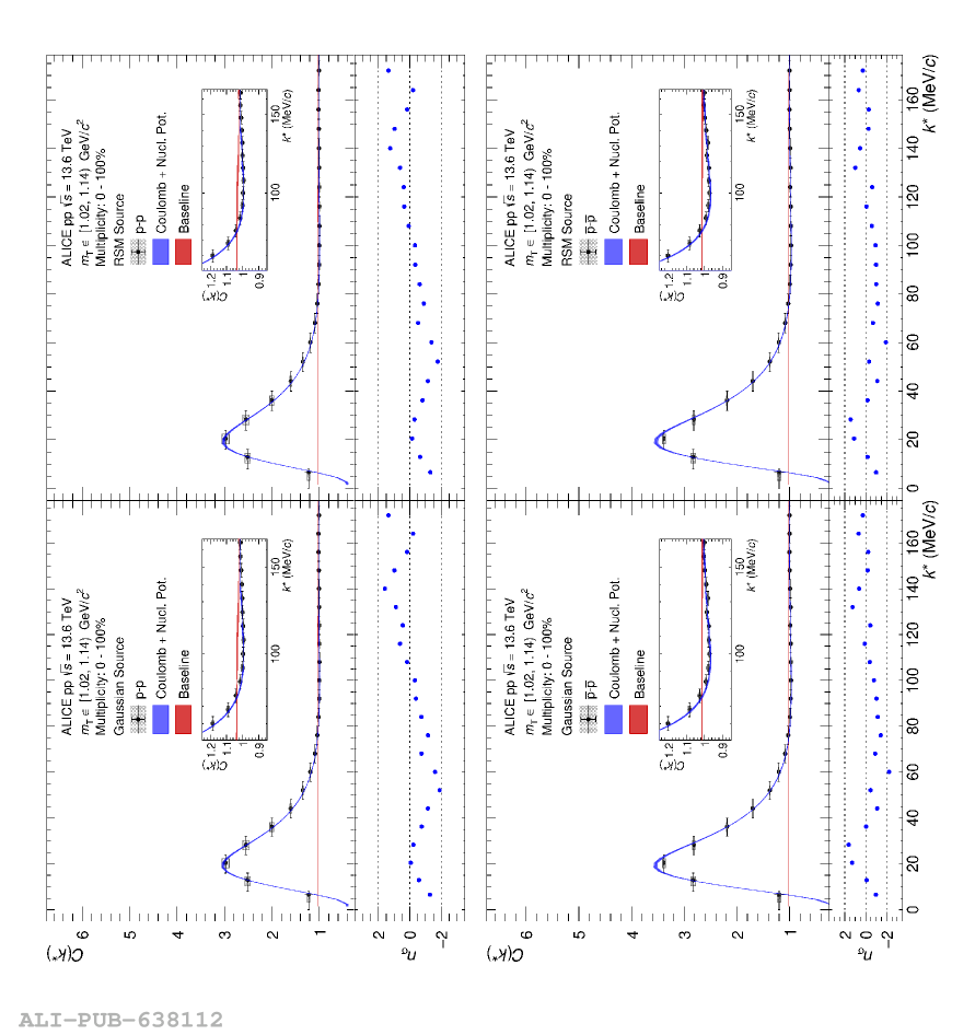 |
Figure A.17
Fits of the multiplicity integrated \pP (upper row) and \ApAp (lower row) correlation functions using the effective Gaussian source (left column) and the RSM (right column) in the \mT range $[1.14, 1.20]\, \si{\gevcc}$. For a detailed description of the panels see \cref{fig:fitsMt0}. | 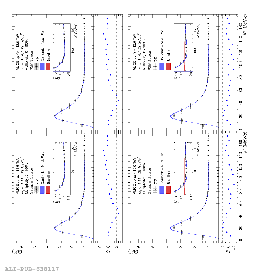 |
Figure A.18
Fits of the multiplicity integrated \pP (upper row) and \ApAp (lower row) correlation functions using the effective Gaussian source (left column) and the RSM (right column) in the \mT range $[1.20, 1.26]\, \si{\gevcc}$. For a detailed description of the panels see \cref{fig:fitsMt0}. | 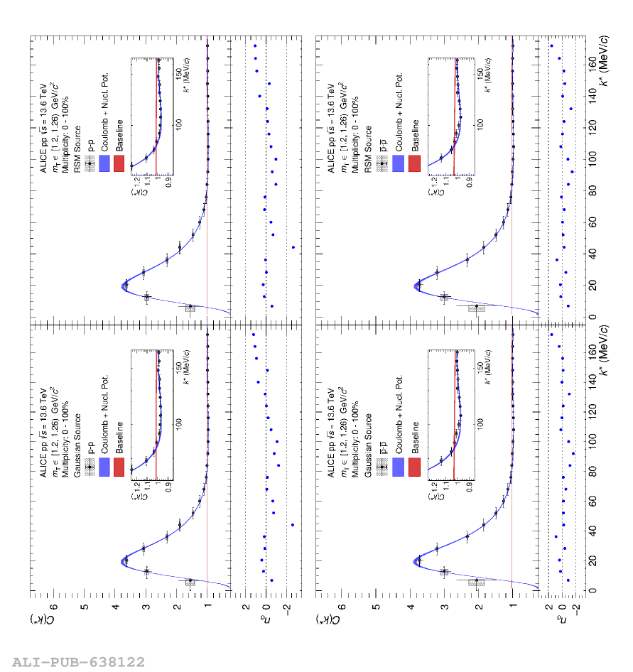 |
Figure A.19
Fits of the multiplicity integrated \pP (upper row) and \ApAp (lower row) correlation functions using the effective Gaussian source (left column) and the RSM (right column) in the \mT range $[1.26, 1.38]\, \si{\gevcc}$. For a detailed description of the panels see \cref{fig:fitsMt0}. | 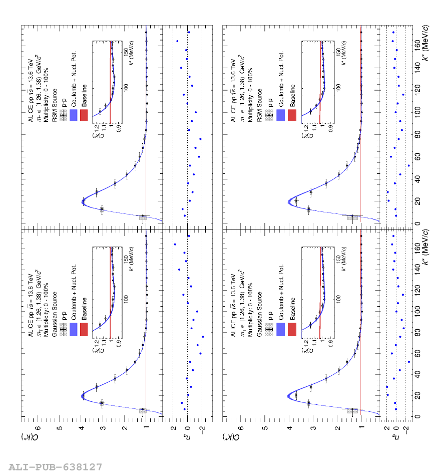 |
Figure A.20
Fits of the multiplicity integrated \pP (upper row) and \ApAp (lower row) correlation functions using the effective Gaussian source (left column) and the RSM (right column) in the \mT range $[1.38, 1.56]\, \si{\gevcc}$. For a detailed description of the panels see \cref{fig:fitsMt0}. | 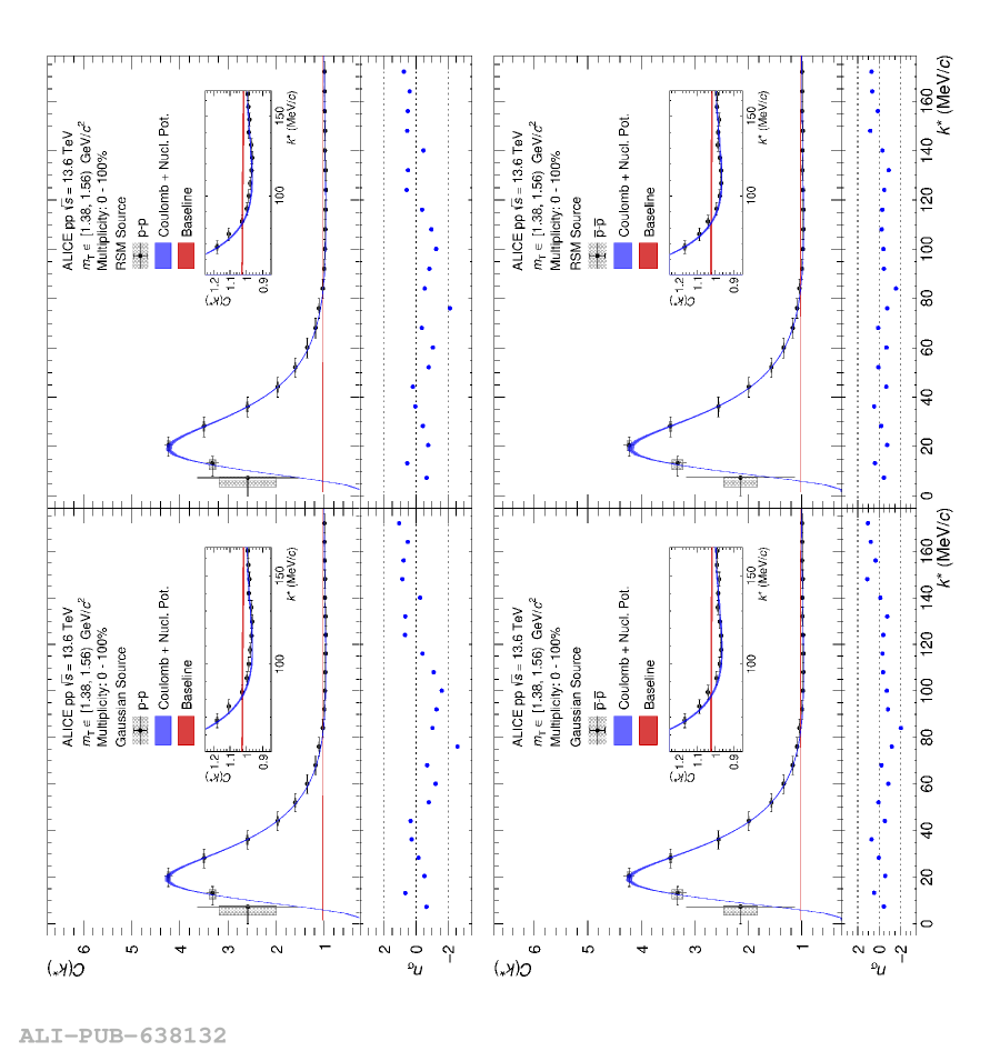 |
Figure A.21
Fits of the multiplicity integrated \pP (upper row) and \ApAp (lower row) correlation functions using the effective Gaussian source (left column) and the RSM (right column) in the \mT range $[1.56, 1.86]\, \si{\gevcc}$. For a detailed description of the panels see \cref{fig:fitsMt0}. | 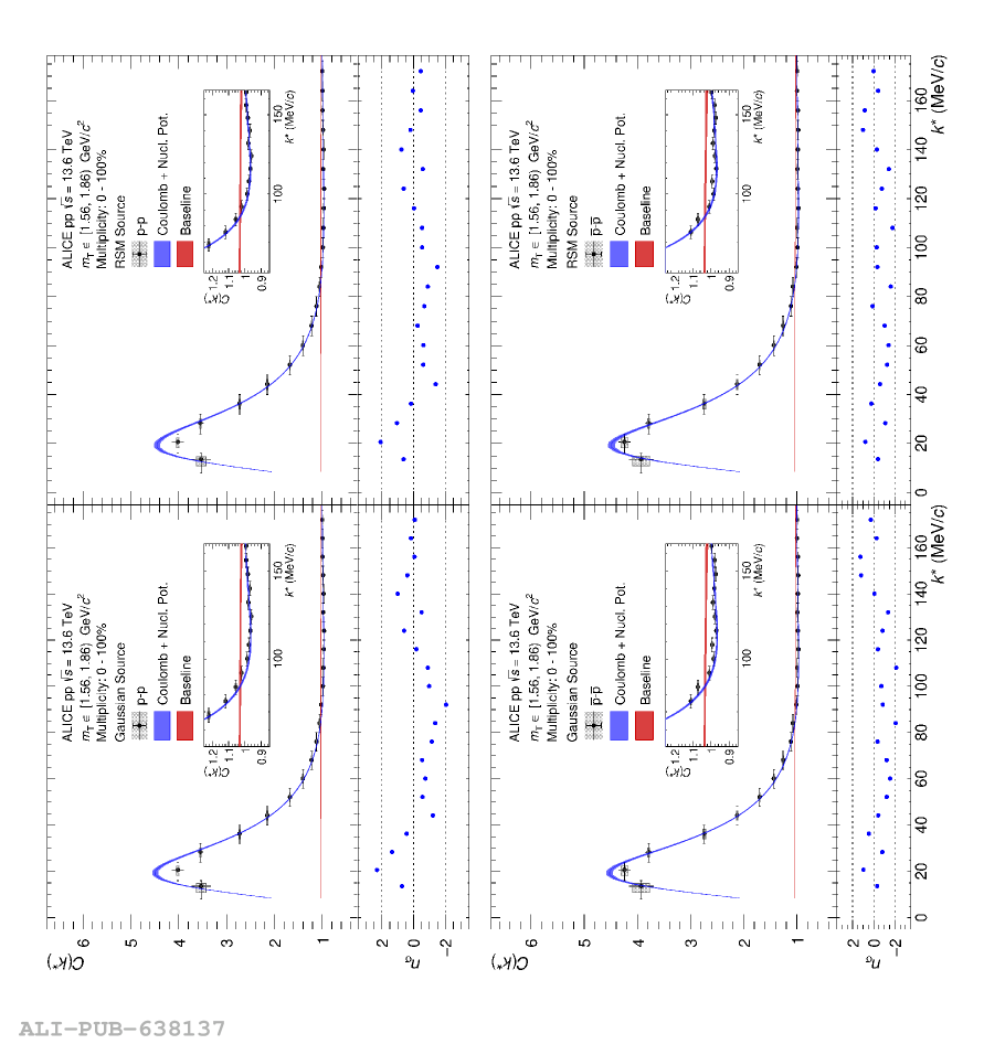 |
Figure A.22
Fits of the multiplicity integrated \pP (upper row) and \ApAp (lower row) correlation functions using the effective Gaussian source (left column) and the RSM (right column) in the \mT range $[1.86, 2.40]\, \si{\gevcc}$. For a detailed description of the panels see \cref{fig:fitsMt0}. | 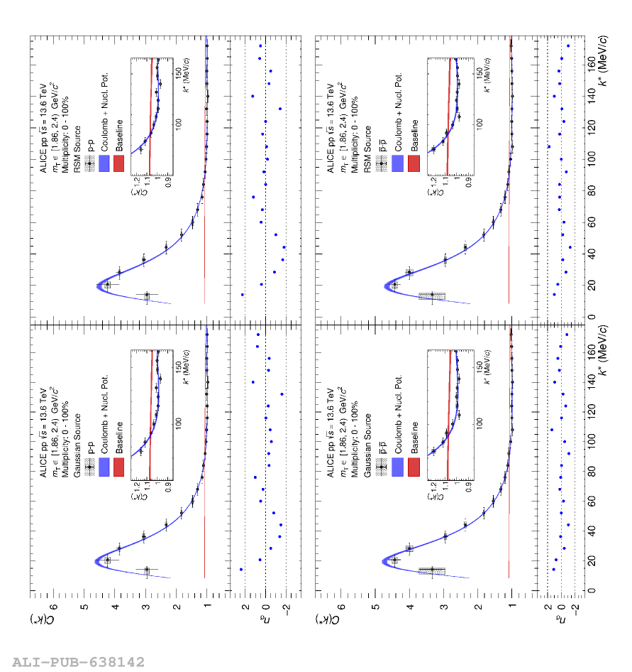 |