The probability to observe a specific number of strange and multi-strange hadrons ($n_s$), denoted as $P(n_s)$, is measured by ALICE at midrapidity ($|y|<~0.5$) in $\sqrt{s} = 5.02$ TeV proton-proton (pp) collisions, dividing events into several multiplicity-density classes. Exploiting a novel technique based on counting the number of strange-particle candidates event-by-event, this measurement allows one to extend the study of strangeness production beyond the mean of the distribution. This constitutes a new test bench for production mechanisms, probing events with a large imbalance between strange and non-strange content. The analysis of a large-statistics data sample makes it possible to extract $P(n_s)$ up to a maximum $n_s$ of 7 for K$^{0}_{\rm s}$, 5 for $Λ$ and $\barΛ$, 4 for $Ξ^-$ and $Ξ^+$, and 2 for $Ω^-$ and $Ω^+$. From this, the probability of producing strange hadron multiplets per event is calculated, thereby enabling the extension of the study of strangeness enhancement to extreme situations where several strange quarks hadronize in a single event at midrapidity. Moreover, comparing hadron combinations with different $\it{u}$ and $\it{d}$ quark compositions and equal overall $s$ quark content, the contribution to the enhancement pattern coming from non-strangeness related mechanisms is isolated. The results are compared with state-of-the-art phenomenological models implemented in commonly used Monte Carlo event generators, including PYTHIA 8 Monash 2013, PYTHIA 8 with QCD-based Color Reconnection and Rope Hadronization (QCD-CR + Ropes), and EPOS LHC, which incorporates both partonic interactions and hydrodynamic evolution. These comparisons show that the new approach dramatically enhances the sensitivity to the different underlying physics mechanisms modeled by each generator.
JHEP 06 (2026) 227
HEP Data
e-Print: arXiv:2511.10413 | PDF | inSPIRE
CERN-EP-2025-257
Figure group
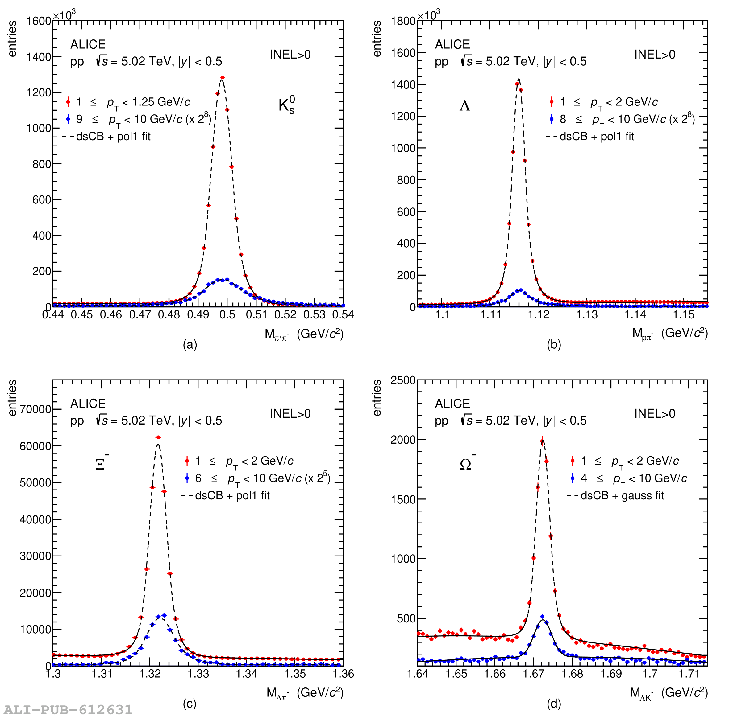
Figure 2
(left) Signal weights at the signal peak position (circles) and at 1$\sigma$ distance from the peak (square markers) for all particles under study as a function of \pt in the \inelgz event class. Dashed lines are shown to guide the eye. (right) Un-corrected multiplicity distribution $n_{\mathrm{S}}^{reco}$ for all particles under study in the \inelgz event class, where statistical uncertainties are evaluated using the sub-samples method and are smaller than the marker size. Particles correspond to full markers, antiparticles to hollow markers. | 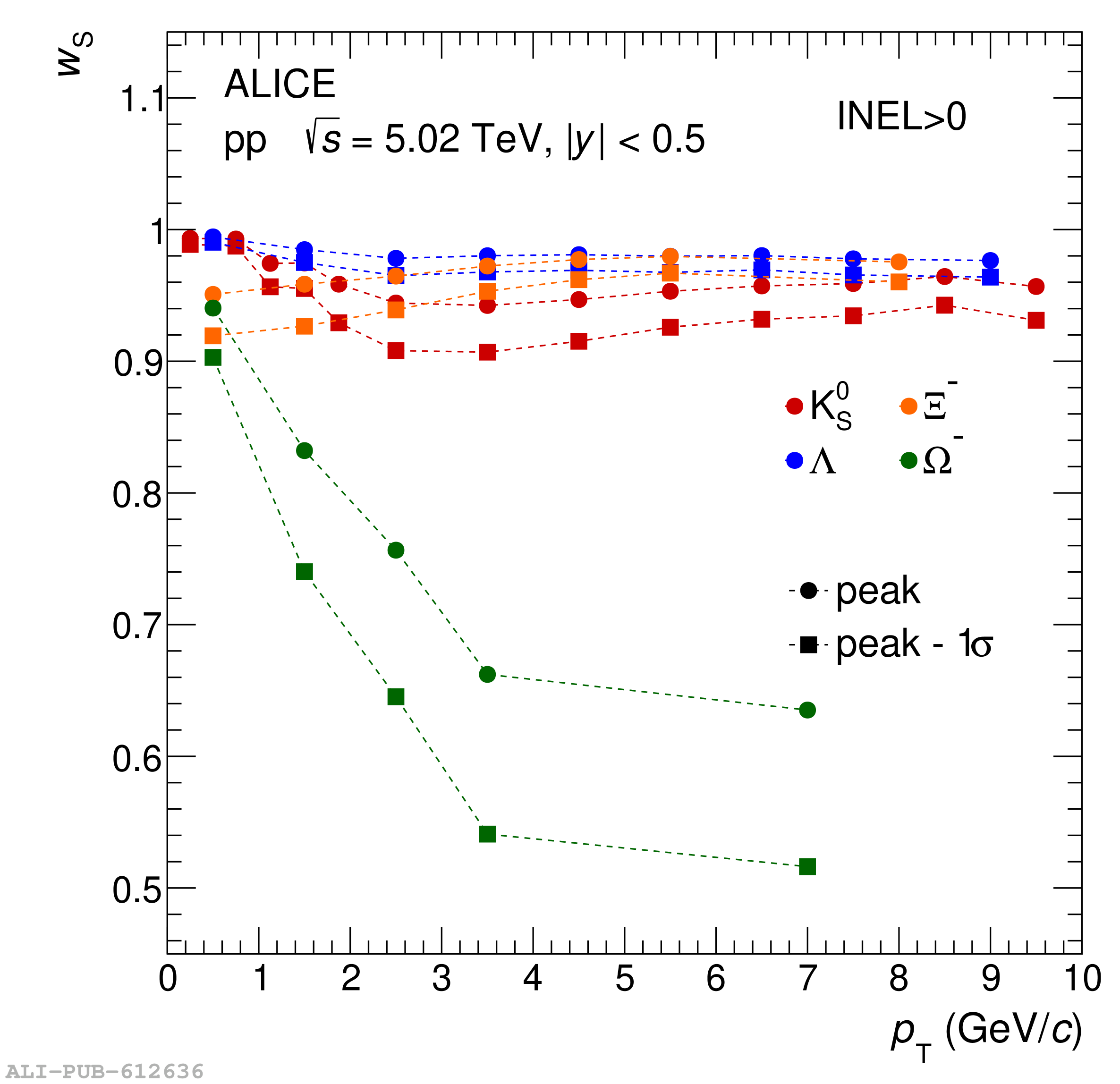 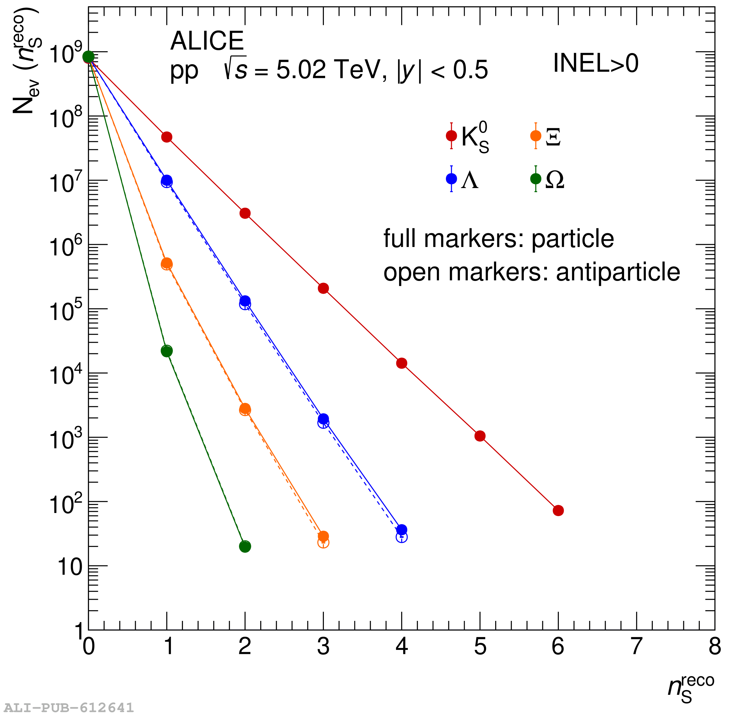 |
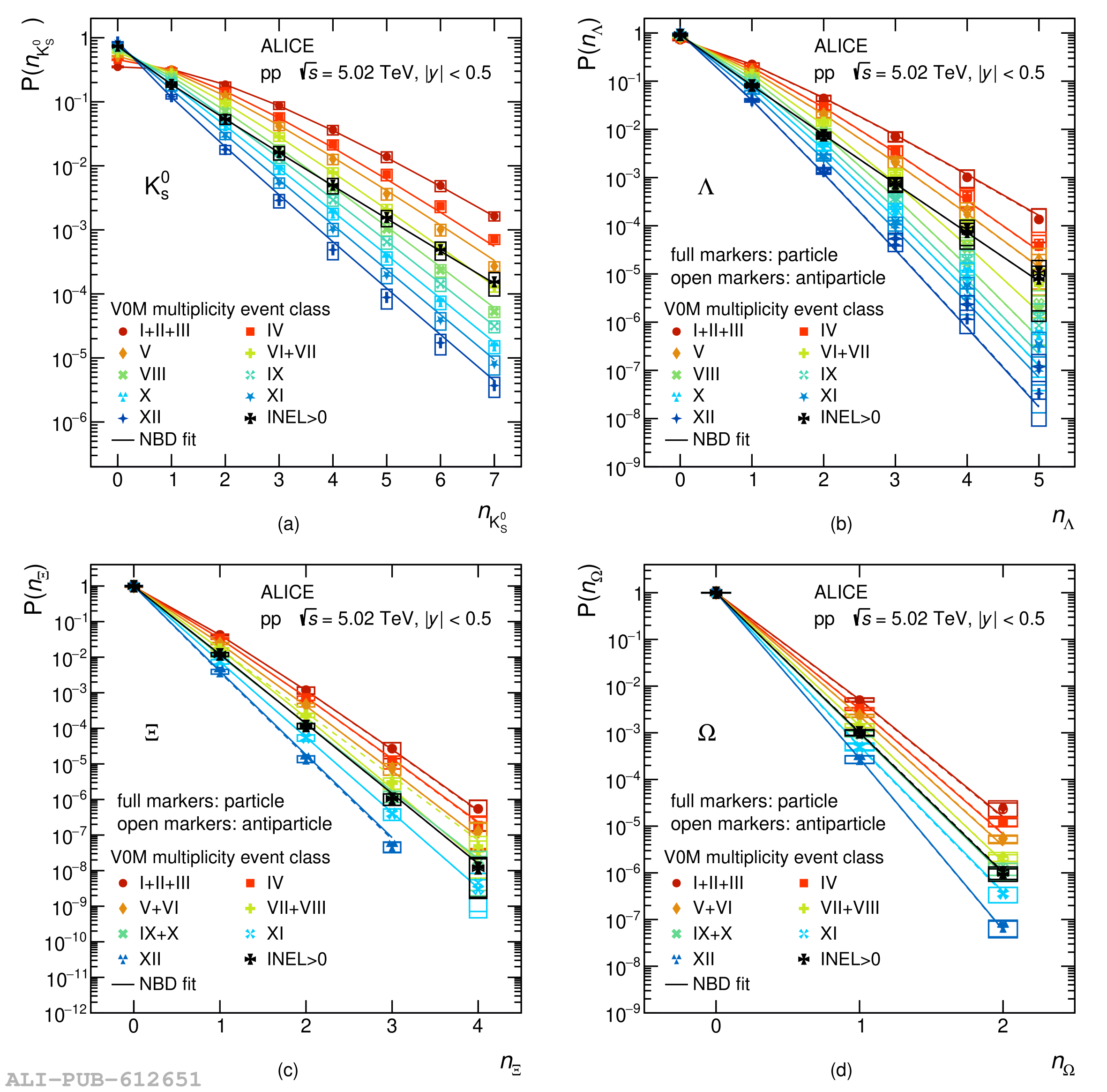
Figure 5
Illustration of the strangeness-induced charged-particle multiplicity bias effect from \pecrr simulation. (left) \dndetamid distribution in the \inelgz, \VZEROM-(I+II+III) and \VZEROM-XII event classes. Open markers are the corresponding \dndetamid resulting from the additional request of at least 5 \kzero in the event. Continuous and dashed vertical lines show the averages of the unbiased and biased multiplicity distributions, respectively. (right) Relative shift in the \avdndeta for all the different \VZEROM event classes when requiring at least one (full markers) or more than one (open markers) strange particles in the event. Lines are shown to guide the eye. | 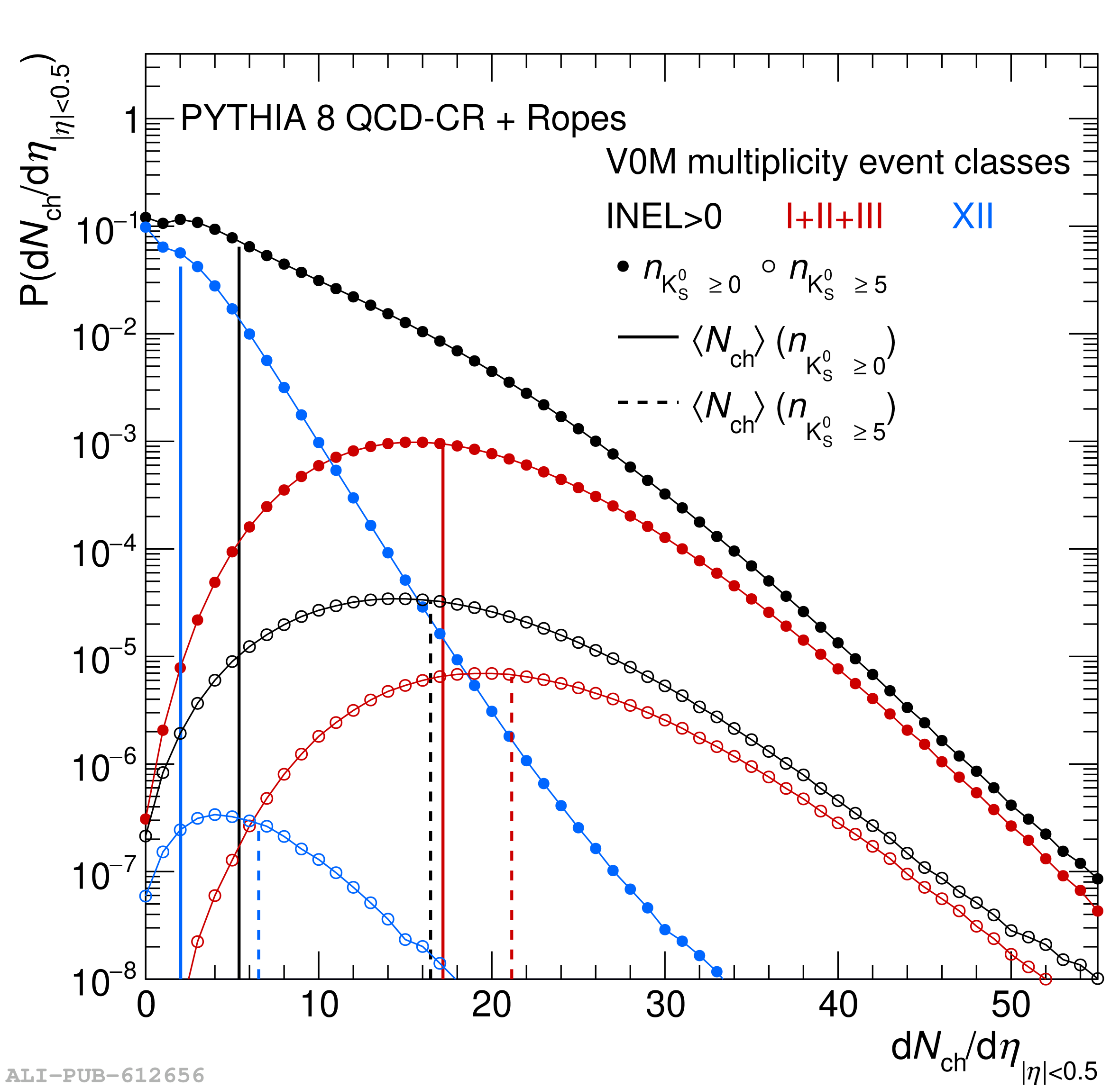 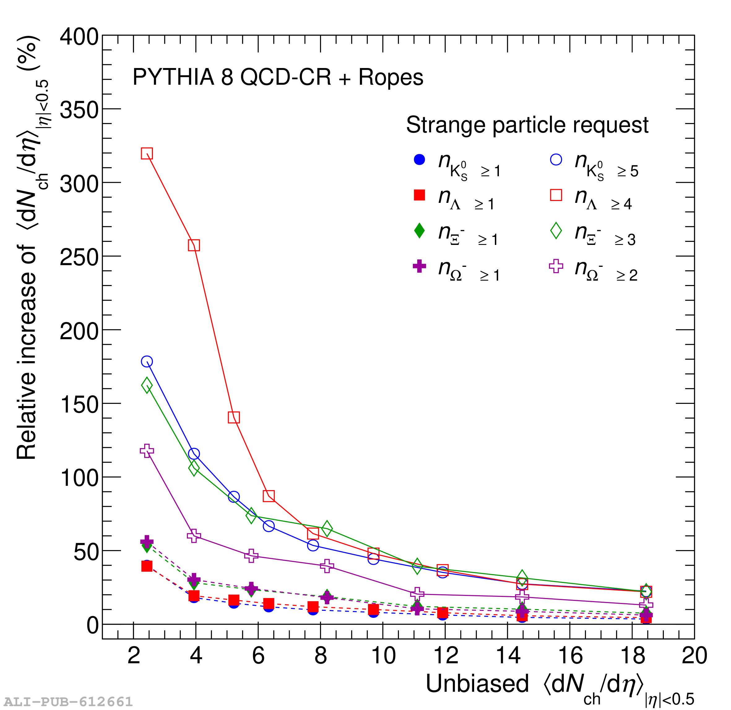 |
Figure 6
Top panel: \ynp{1}{S} and \ynp{n>1}{S}/\ynp{1}{S} in the \inelgz event class for all particles under study. Model predictions by \pem, \pecrr and \eplhc are shown as dotted, continuous, and dashed lines, respectively. Central panel: deviation between data and models in units of the total uncertainty. Bottom panel: deviation from independent production hypothesis for both data and models. Results for different particles are shifted in $x$ to improve visibility. | 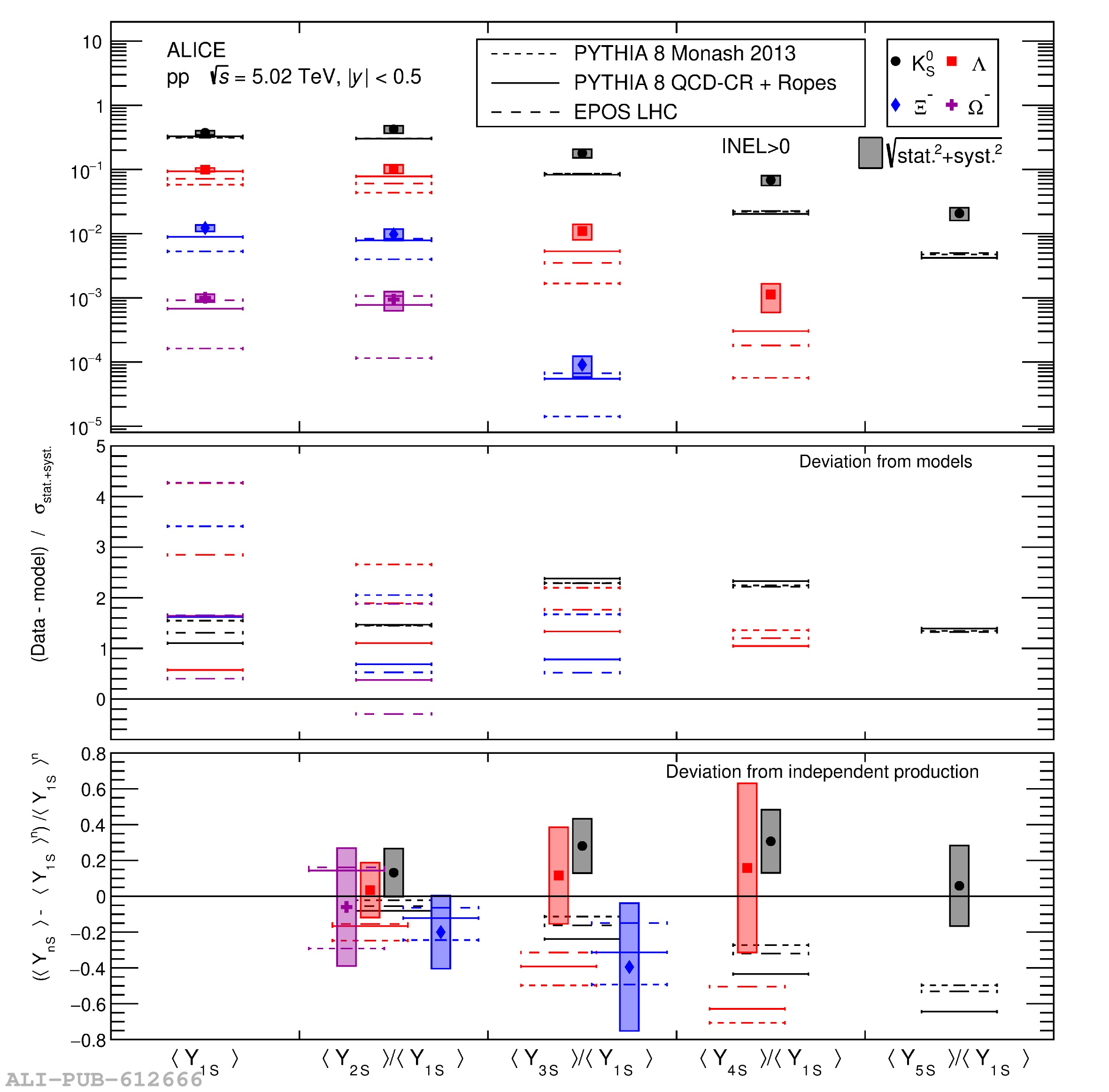 |
Figure 7
Multiple strange-hadron production yields as a function of the unbiased average charged-particle multiplicity \dndetaNew for \kzero (a), \lmb (b), \XiNosign (c) and \OmNosign (d). Full markers correspond to particles, open markers to antiparticles. Model predictions are reported for \pem, \pecrr and \eplhc as dotted, continuous and dashed lines respectively. | 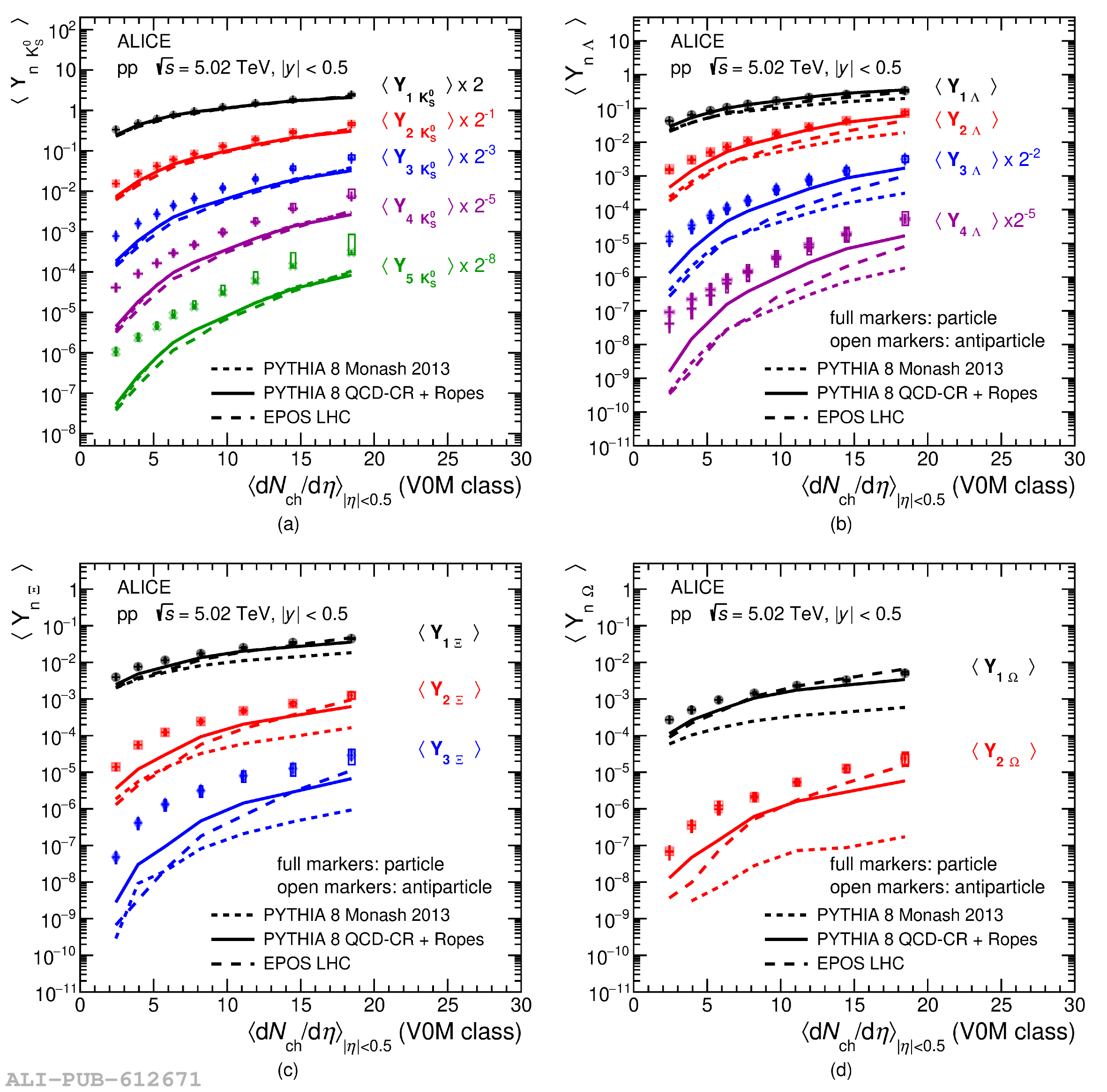 |
Figure 8
Ratios between the average production yield of $m$ baryons, \ynp{m\,}{baryon}, and $n$ \kzero, \ynp{n\,}{\kzero}, as a function of the unbiased average charged-particle multiplicity, \dndetaNew. The case $m=3$, corresponding to \ynp{3}{\X}, is illustrated with full markers, while $m=2$, corresponding to \ynp{2}{\Om}, is shown with open markers. The value of $n$ ranges from 1 to 4, from top to bottom, respectively. Open markers are shifted to the right by 10\% to enhance visibility. | 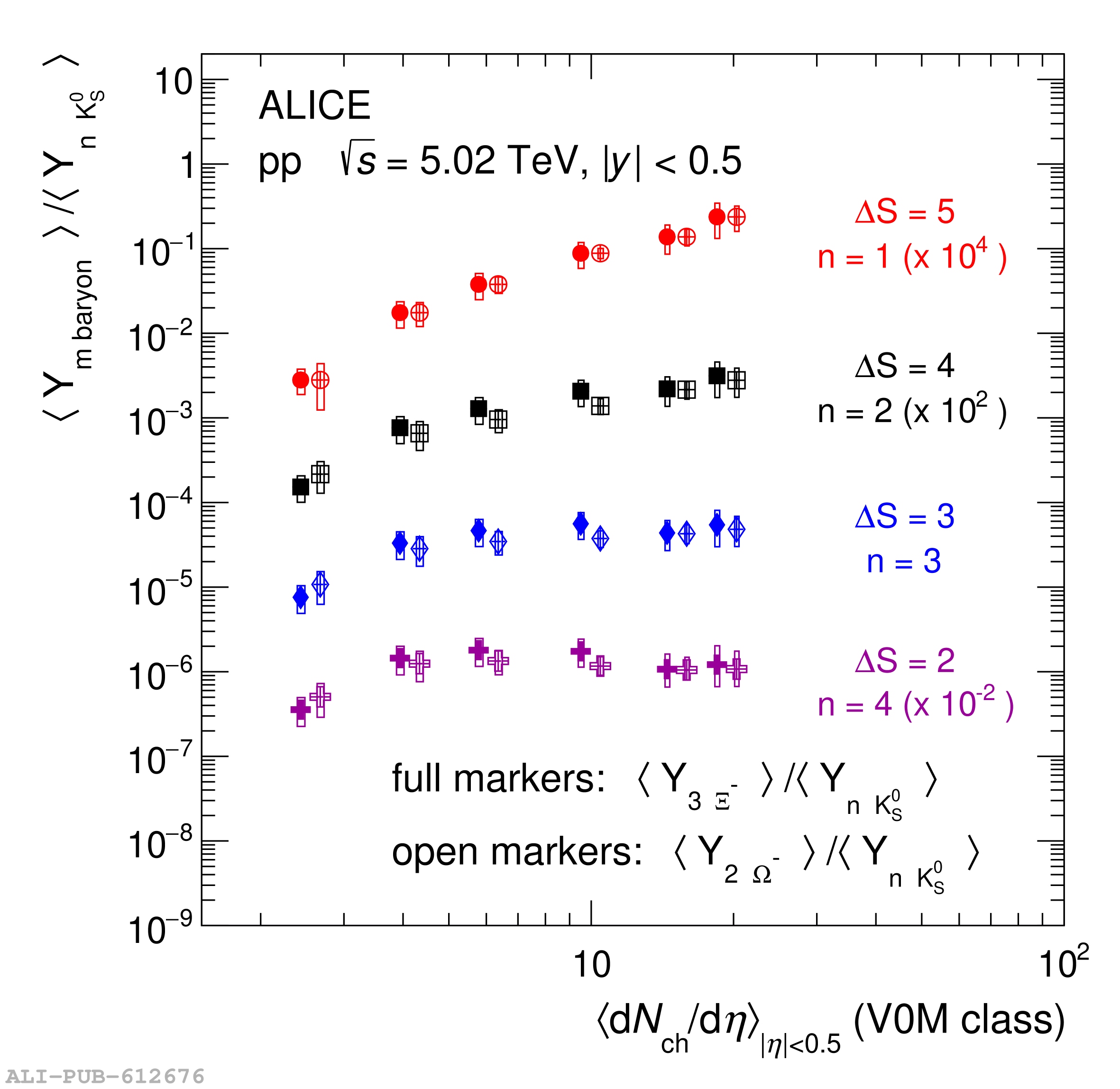 |
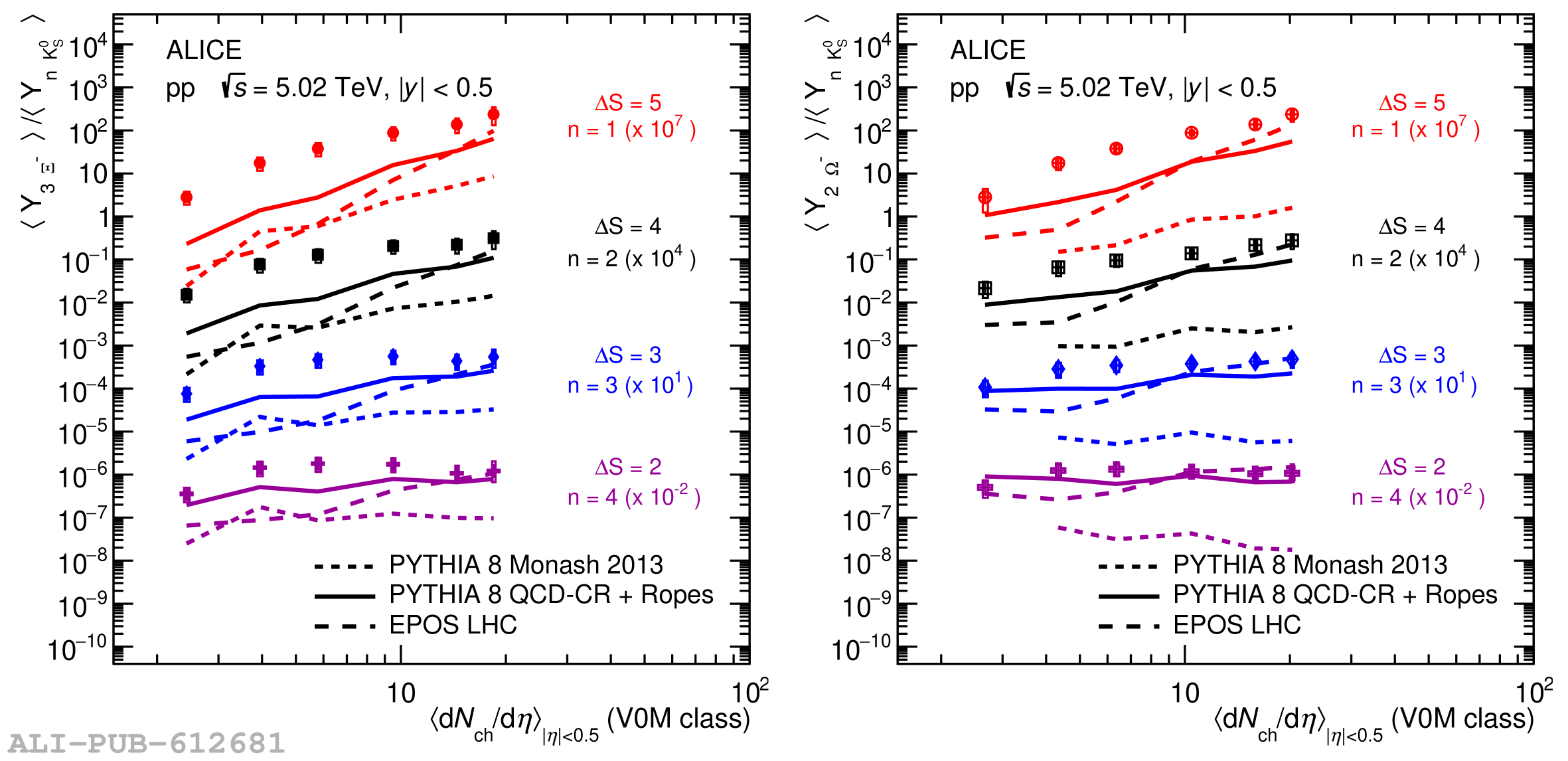
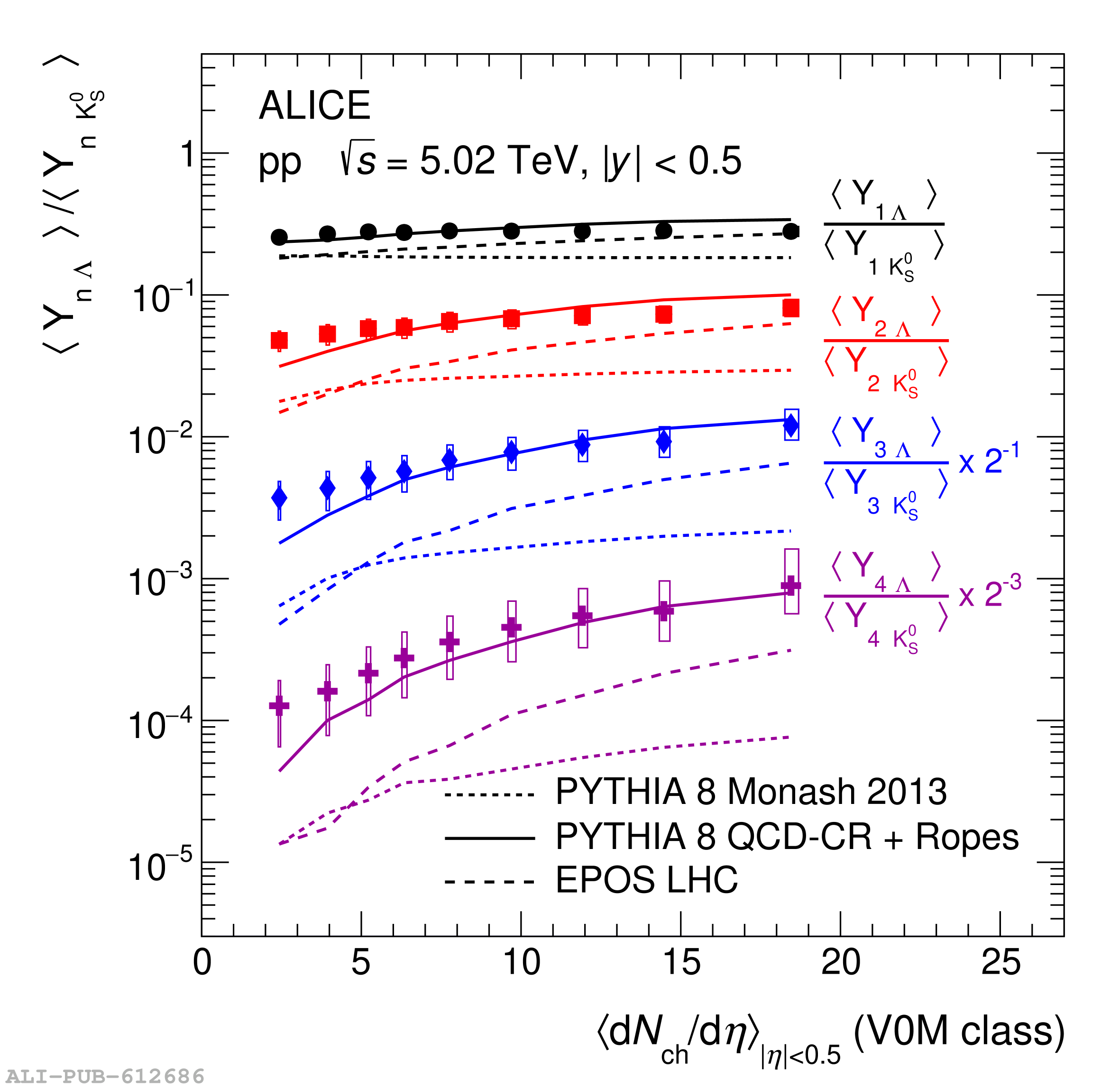
Figure 11
Ratios of the average production yield of $m$ multi-strange baryons \ynp{m\,}{baryon}, to those of $n$ single-strange particles, \ynp{n\,}{\kzero} (left) and \ynp{n\,}{\lmb} (right), as a function of the unbiased average charged-particle multiplicity, \dndetaNew. The measurements are compared to MC predictions from \pem (dotted lines), \pecrr (continuous lines) and \eplhc (dashed lines). (left) \ynp{1}{\X}/\ynp{2}{\kzero}, \ynp{1}{\Om}/\ynp{3}{\kzero} and \ynp{2}{\X}/\ynp{4}{\kzero} from top to bottom respectively. (right) \ynp{1}{\X}/\ynp{2}{\lmb}, \ynp{1}{\Om}/\ynp{3}{\lmb} and \ynp{2}{\X}/\ynp{4}{\lmb} from top to bottom respectively. | 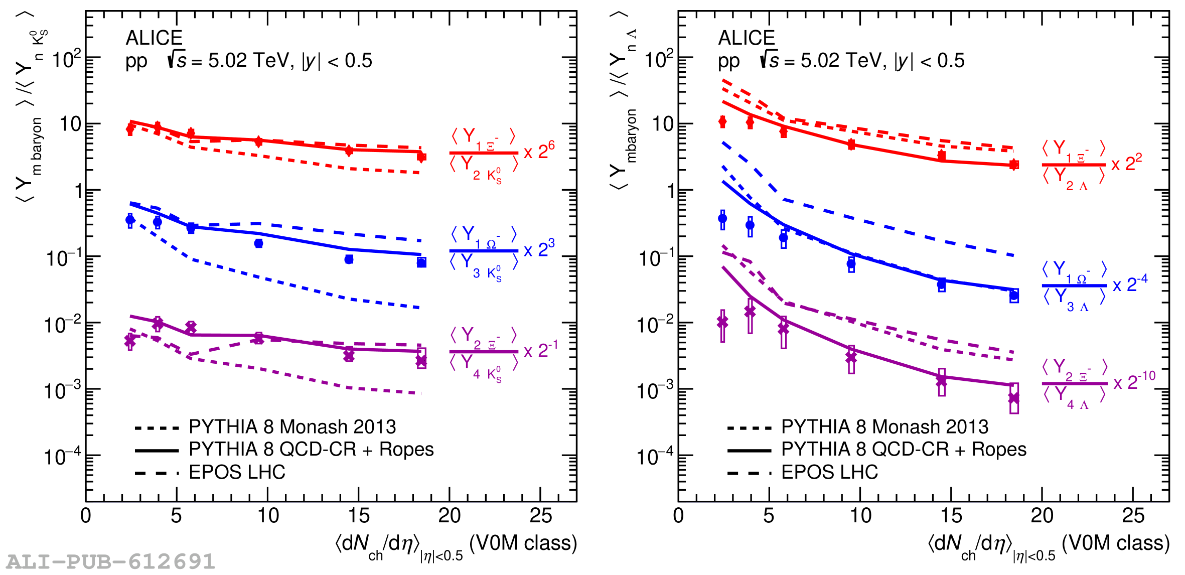 |