The multi-strange baryon yields in Pb--Pb collisions have been shown to exhibit an enhancement relative to pp reactions. In this work, $\Xi$ and $\Omega$ production rates have been measured with the ALICE experiment as a function of transverse momentum, ${p_{\rm T}}$, in p-Pb collisions at a centre-of-mass energy of ${\sqrt{s_{\rm NN}}}$ = 5.02 TeV. The results cover the kinematic ranges 0.6 GeV/$c<~{p_{\rm T}} <~$7.2 GeV/$c$ and 0.8 GeV/$c<~{p_{\rm T}}<~$ 5 GeV/$c$, for $\Xi$ and $\Omega$ respectively, in the common rapidity interval -0.5 $<~{y_{\rm CMS}}<~$ 0. Multi-strange baryons have been identified by reconstructing their weak decays into charged particles. The ${p_{\rm T}}$ spectra are analysed as a function of event charged-particle multiplicity, which in p-Pb collisions ranges over one order of magnitude and lies between those observed in pp and Pb-Pb collisions. The measured ${p_{\rm T}}$ distributions are compared to the expectations from a Blast-Wave model. The parameters which describe the production of lighter hadron species also describe the hyperon spectra in high multiplicity p-Pb. The yield of hyperons relative to charged pions is studied and compared with results from pp and Pb-Pb collisions. A statistical model is employed, which describes the change in the ratios with volume using a canonical suppression mechanism, in which the small volume causes a species-dependent relative reduction of hadron production. The calculations, in which the magnitude of the effect depends on the strangeness content, show good qualitative agreement with the data.
Phys. Lett. B 758 (2016) 389-401
HEP Data
e-Print: arXiv:1512.07227 | PDF | inSPIRE
CERN-PH-EP-2015-327
Figure 1
Invariant mass distributions of the $\Xi^{-}$ and $\Omega^{-}$ in the 1.1-1.2 \GeVc and 1.2-1.6 \GeVc \pt\ bins respectively, fitted with a Gaussian peak and linear background (dashed red curves). The distributions for highest (left) and lowest (right) multiplicity classes are shown. The fits only serve to illustrate the peak position with respect to which the bands were defined and the linear background assumption for the applied signal extraction method. | 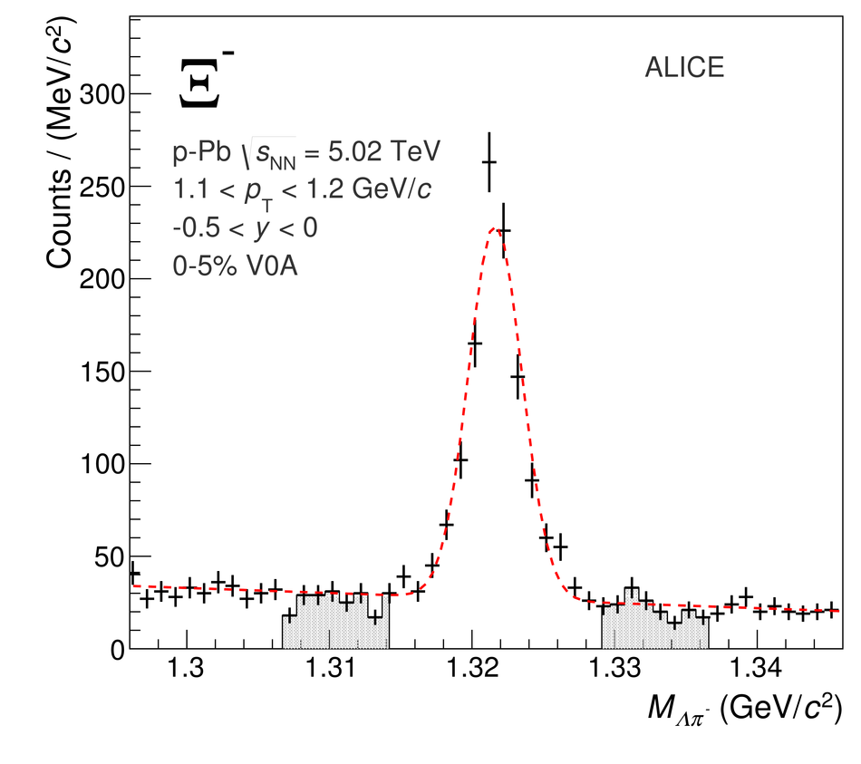 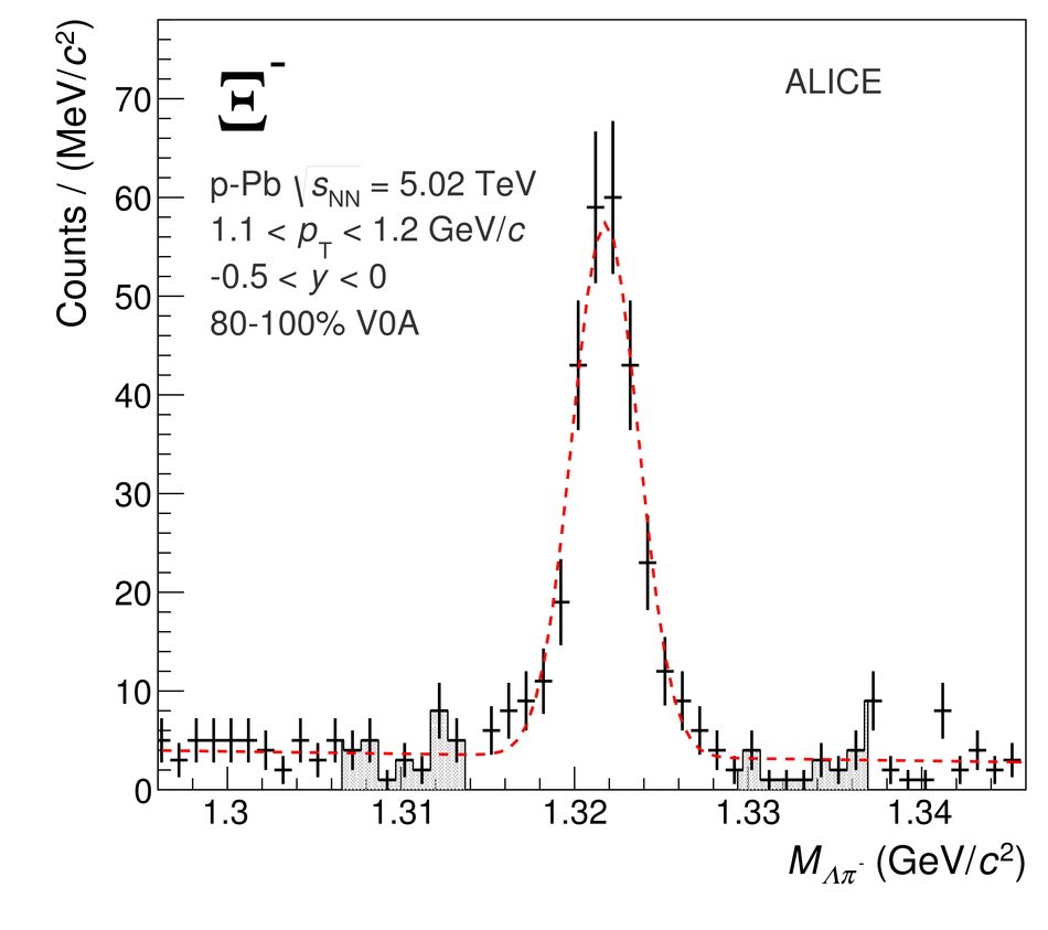 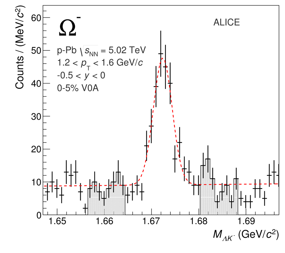 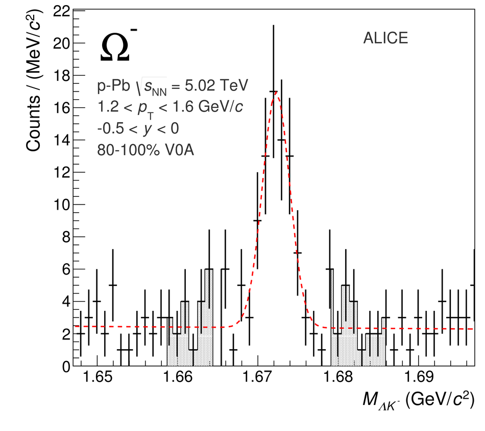 |
Figure 2
(colour online) Invariant \pt-differential yields of (\X+\Ix) and (\Om+\Mo) in different multiplicity classes. Data have been scaled by successive factors of 2 for better visibility. Statistical (bars), full systematic (boxes) and uncorrelated across multiplicity (transparent boxes) uncertainties are plotted. The dashed curves represent Blast-Wave fits to each individual distribution. | 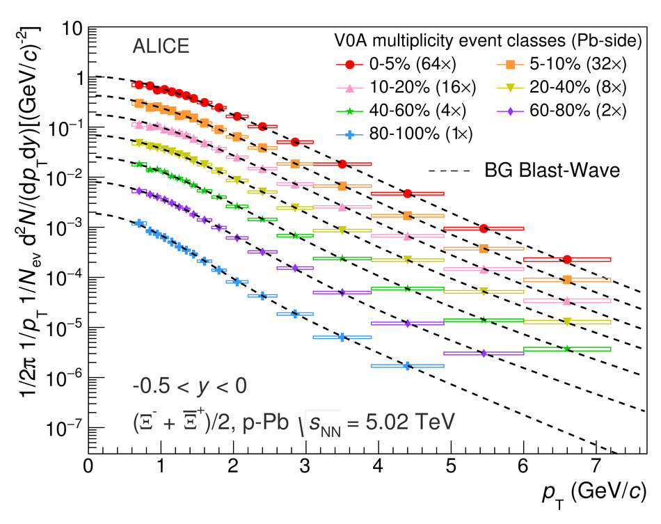 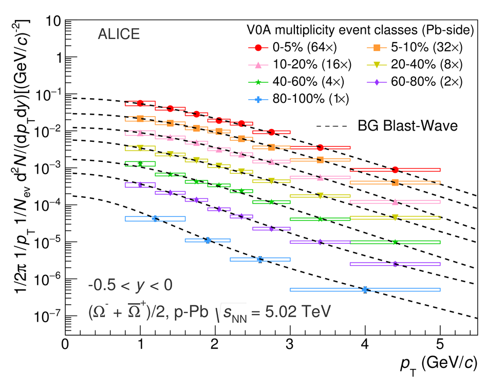 |
Figure 3
(colour online) (\X+\Ix) and (\Om+\Mo) \pt\ spectra in the 0--5$\%$ (left) and 80--100$\%$ (right) multiplicity classes compared to predictions from the BG-BW model (upper panels) with the ratios on a linear scale (lower panels). The parameters are based on simultaneous fits to lighter hadrons . See text for details. |  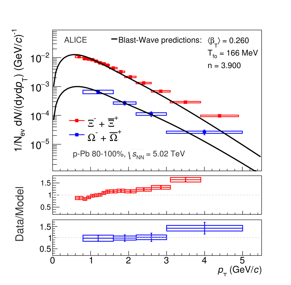 |
Figure 4
(colour online) (\X+\Ix)/(\pip+\pim) (left) and (\Om+\Mo)/(\pip+\pim) (right) ratios as a function of $\avg{\dNdeta}$ for all three colliding systems. The ratios for the seven multiplicity classes in \pPb\ data lie between the Minimum Bias pp (\s = 900 GeV and \s = 7 TeV ) and peripheral \PbPb\ results. The \PbPb\ points represent, from left to right, the 60-80$\%$, 40-60$\%$, 20-40$\%$ and 10-20$\%$ and 0-10$\%$ centrality classes. The chemical equilibrium predictions by the GSI-Heidelberg and the \thermus 2.3 models are represented by the horizontal lines. | 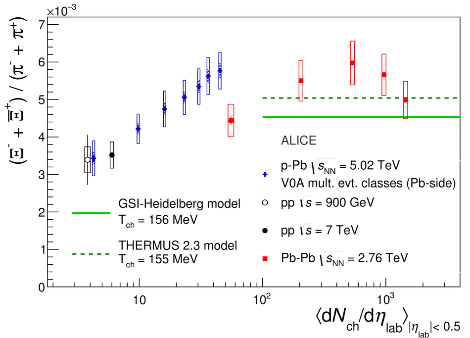 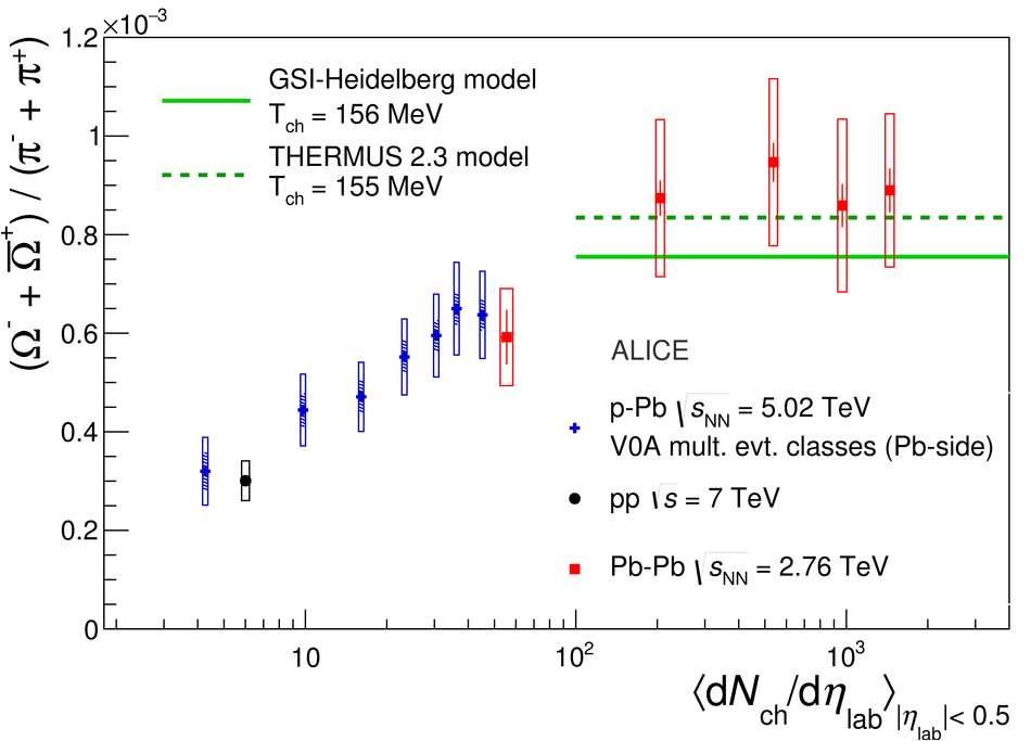 |
Figure 5
(colour online) Hyperon to pion ratios as a function of pion yields for pp, \pPb\ and \PbPb\ colliding systems compared to the \thermus\ strangeness suppression model prediction, in which only the system size is varied. The h/$\pi$ are the ratios of the particle and antiparticle sums, except for the 2$\Lambda$/($\pi^{-}+\pi^{+}$) data points in pp , \pPb and \PbPb . All values are normalised to the high multiplicity limit, which is given by the mean of the 0-60\% highest multiplicity \PbPb measurements for the data and by the GC limit for the model. |  |