The angular correlations between charged $\Xi$ baryons and associated identified hadrons (pions, kaons, protons, $\Lambda$ baryons, and $\Xi$ baryons) are measured in pp collisions at $\sqrt{s} = 13$ TeV with the ALICE detector to give insight into the particle production mechanisms and balancing of quantum numbers on the microscopic level. In particular, the distribution of strangeness is investigated in the correlations between the doubly-strange $\Xi$ baryon and mesons and baryons that contain a single strange quark, K and $\Lambda$. As a reference, the results are compared to $\Xi\pi$ and $\Xi\mathrm{p}$ correlations, where the associated mesons and baryons do not contain a strange valence quark. These measurements are expected to be sensitive to whether strangeness is produced through string breaking or in a thermal production scenario. Furthermore, the multiplicity dependence of the correlation functions is measured to look for the turn-on of additional particle production mechanisms with event activity. The results are compared to predictions from the string-breaking model PYTHIA 8, including tunes with baryon junctions and rope hadronisation enabled, the cluster hadronisation model HERWIG 7, and the core-corona model EPOS-LHC. While some aspects of the experimental data are described quantitatively or qualitatively by the Monte Carlo models, no model can match all features of the data. These results provide stringent constraints on the strangeness and baryon number production mechanisms in pp collisions.
JHEP 09 (2024) 102
e-Print: arXiv:2308.16706 | PDF | inSPIRE
CERN-EP-2023-198
Figure group
Figure 1
$\Xi\pi$ (top row) and $\Xi\mathrm{K}$ (bottom row) per-trigger yields in $(\Delta y,\Delta\varphi)$ for particle pair combinations with the opposite (left column) and same (right column) electric charge, measured in pp collisions at $\sqrt{s} = 13$ TeV. | 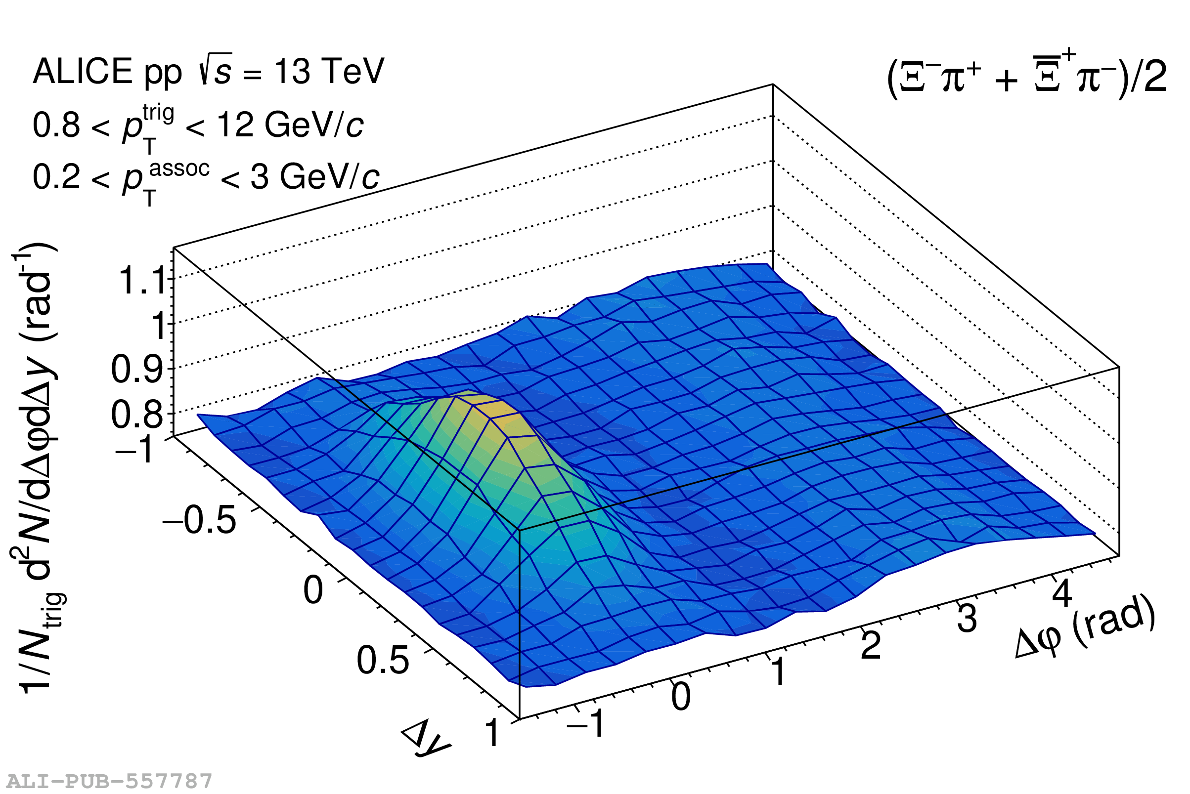 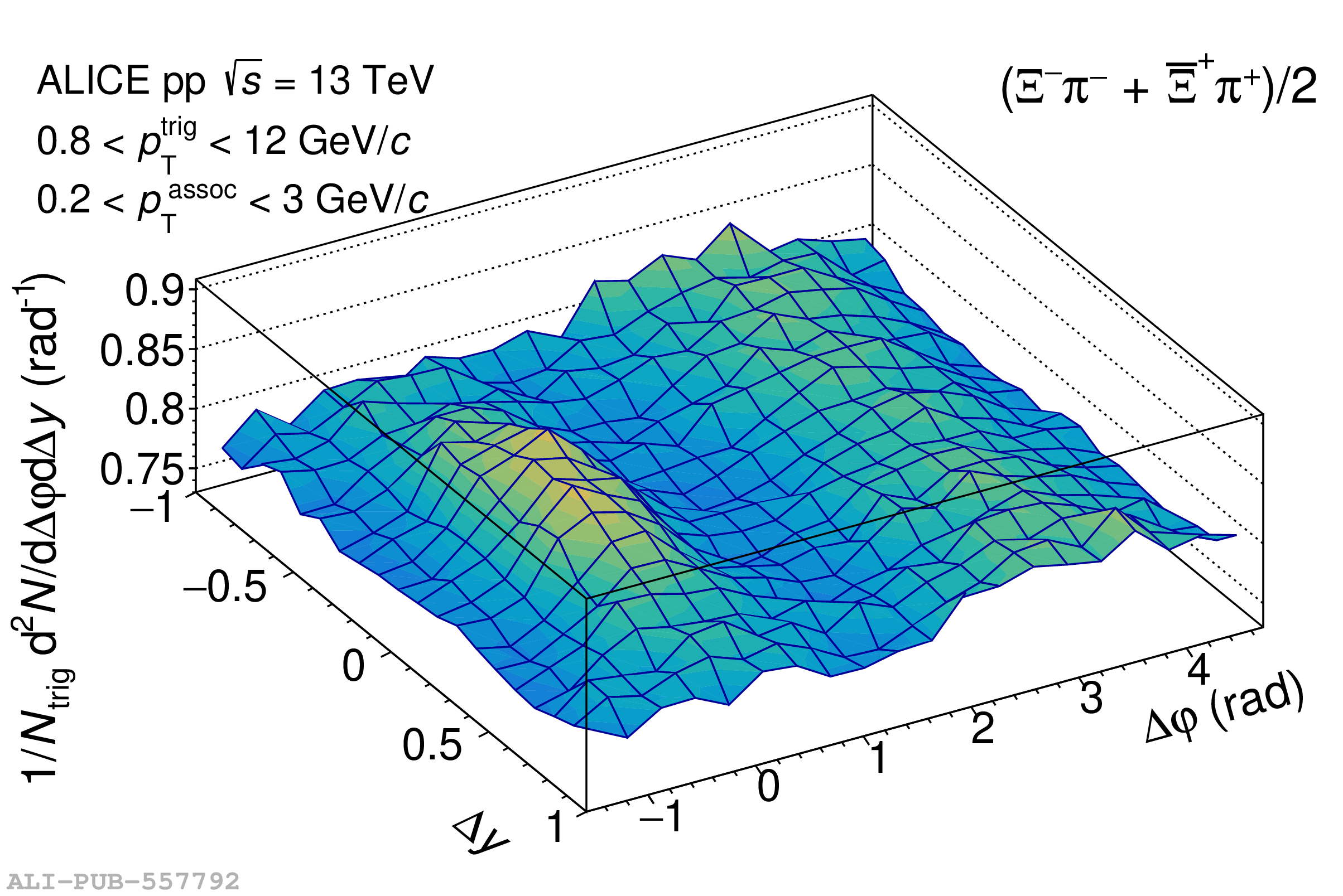 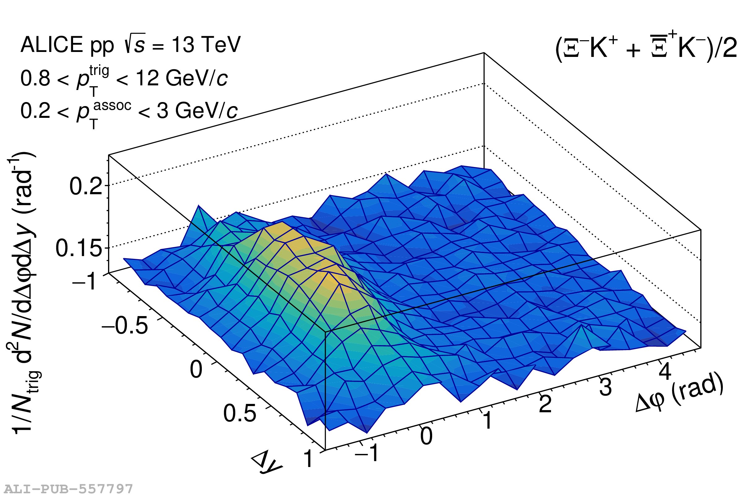 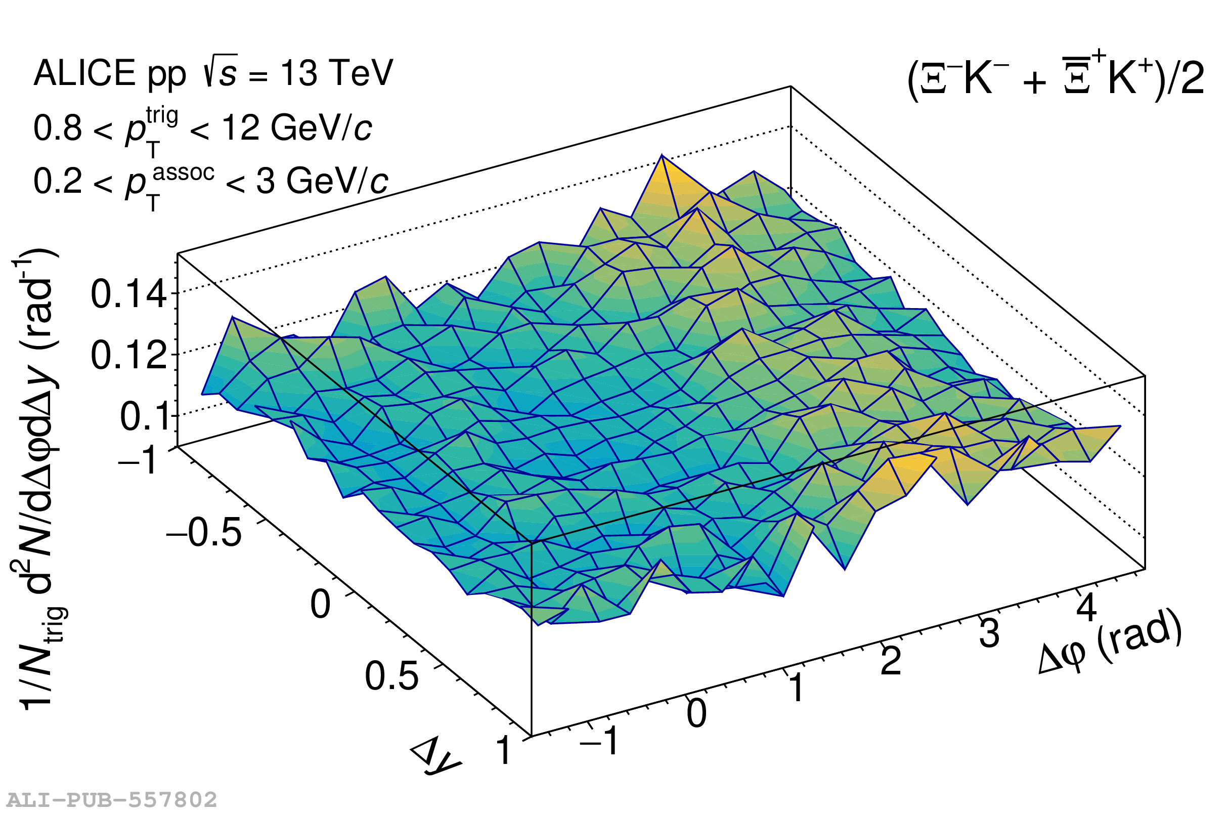 |
Figure 2
$\Xi^-\pi^+$ and $\Xi^-\pi^-$ (and charge conjugate) correlation functions projected onto $\Delta\varphi$ ($|\Delta y| < 1$, left), the near-side on $\Delta y$ ($|\Delta\varphi| < \pi/2$, middle), and the away-side on $\Delta y$ ($\pi/2 < \Delta\varphi < 3\pi/2$, right). Opposite-sign ($\Xi^{-}\pi^{+}+\overline{\Xi}^{+}\pi^{-}$) correlations are shown in grey squares, the same-sign ($\Xi^{-}\pi^{-}+\overline{\Xi}^{+}\pi^{+}$) correlations are black circles; the OS$-$SS difference is displayed in the bottom panels. Statistical and systematic uncertainties are represented by bars and boxes, respectively. The ALICE data are compared with the following models: PYTHIA 8 Monash tune (blue), PYTHIA 8 with junctions enabled (green), PYTHIA 8 with junctions and ropes (yellow), EPOS-LHC (red), and HERWIG 7 (pink). | 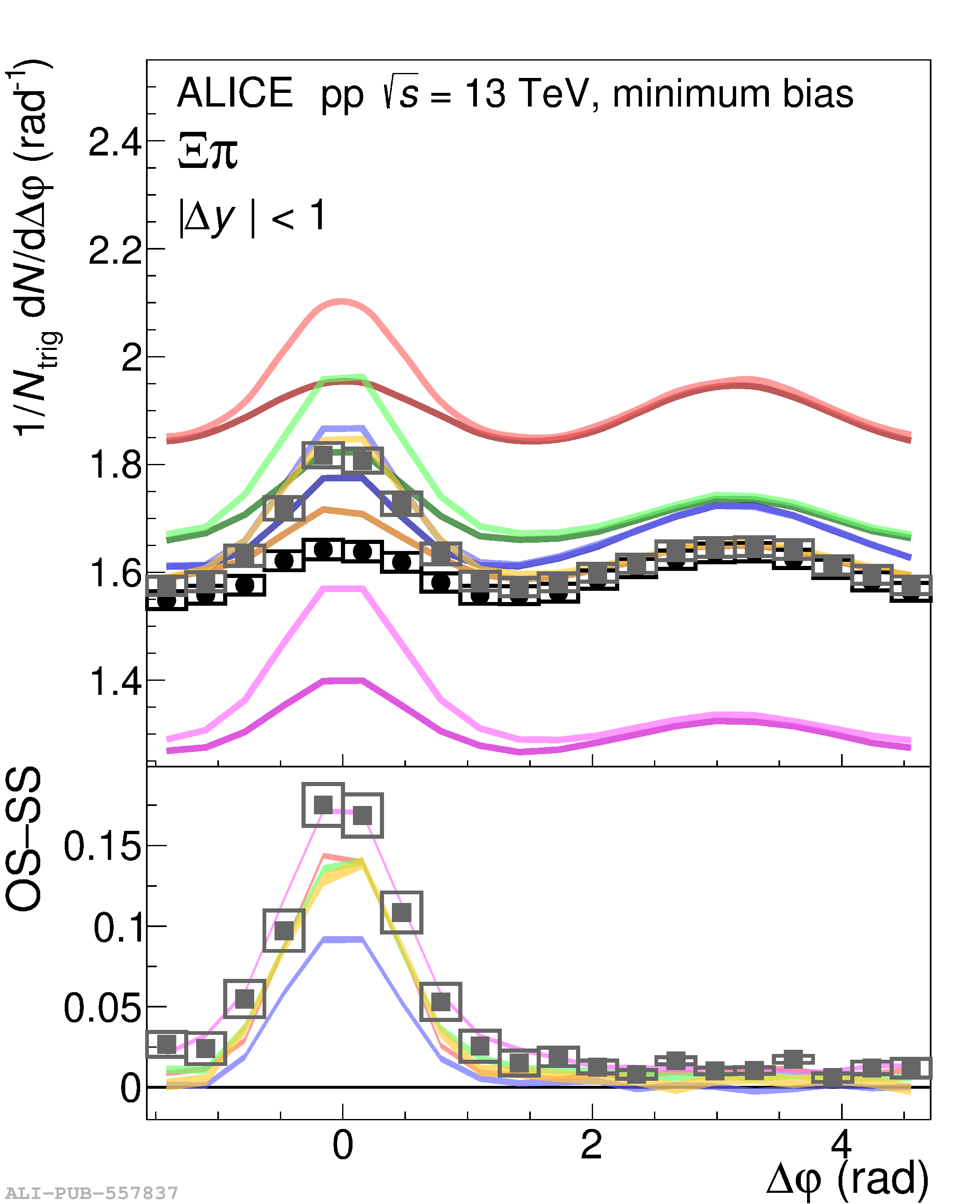 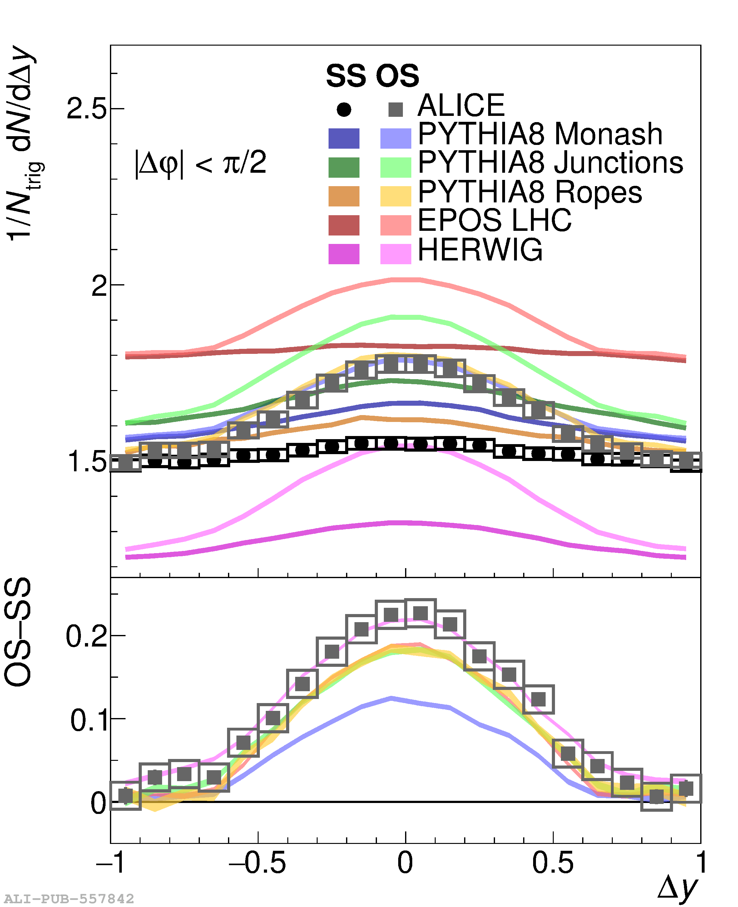 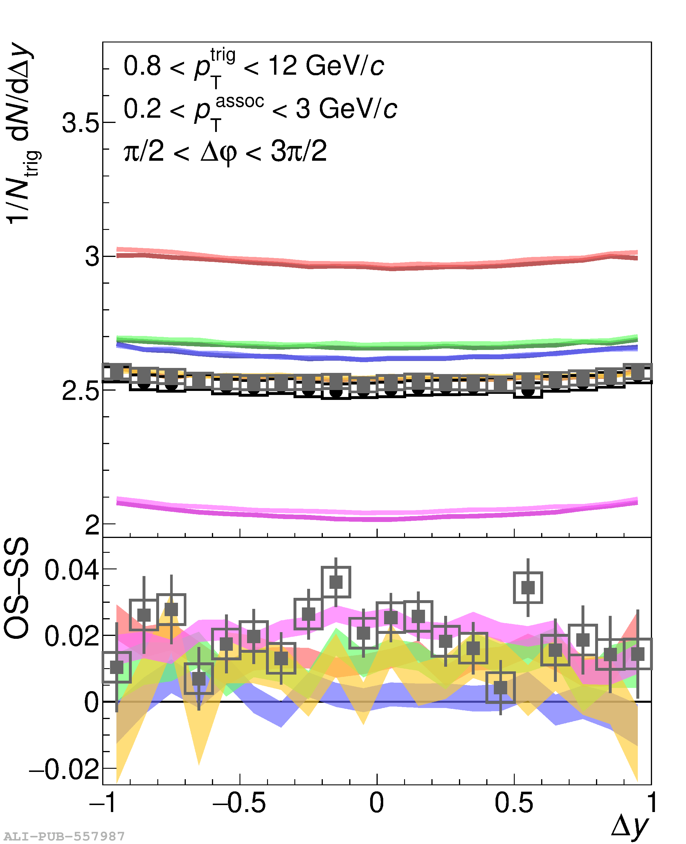 |
Figure 3
$\Xi^-\mathrm{K}^+$ and $\Xi^-\mathrm{K}^-$ (and charge conjugate) correlation functions projected onto $\Delta\varphi$ ($|\Delta y| < 1$, left), the near-side on $\Delta y$ ($|\Delta\varphi| < \pi/2$, middle), and the away-side on $\Delta y$ ($\pi/2 < \Delta\varphi < 3\pi/2$, right). Opposite-sign ($\Xi^{-}\mathrm{K}^{+}+\overline{\Xi}^{+}\mathrm{K}^{-}$) correlations are shown in grey squares, the same-sign ($\Xi^{-}\mathrm{K}^{-}+\overline{\Xi}^{+}\mathrm{K}^{+}$) correlations are black circles; the OS$-$SS difference is displayed in the bottom panels. Statistical and systematic uncertainties are represented by bars and boxes, respectively. The ALICE data are compared with the following models: PYTHIA 8 Monash tune (blue), PYTHIA 8 with junctions enabled (green), PYTHIA 8 with junctions and ropes (yellow), EPOS-LHC (red), and HERWIG 7 (pink). | 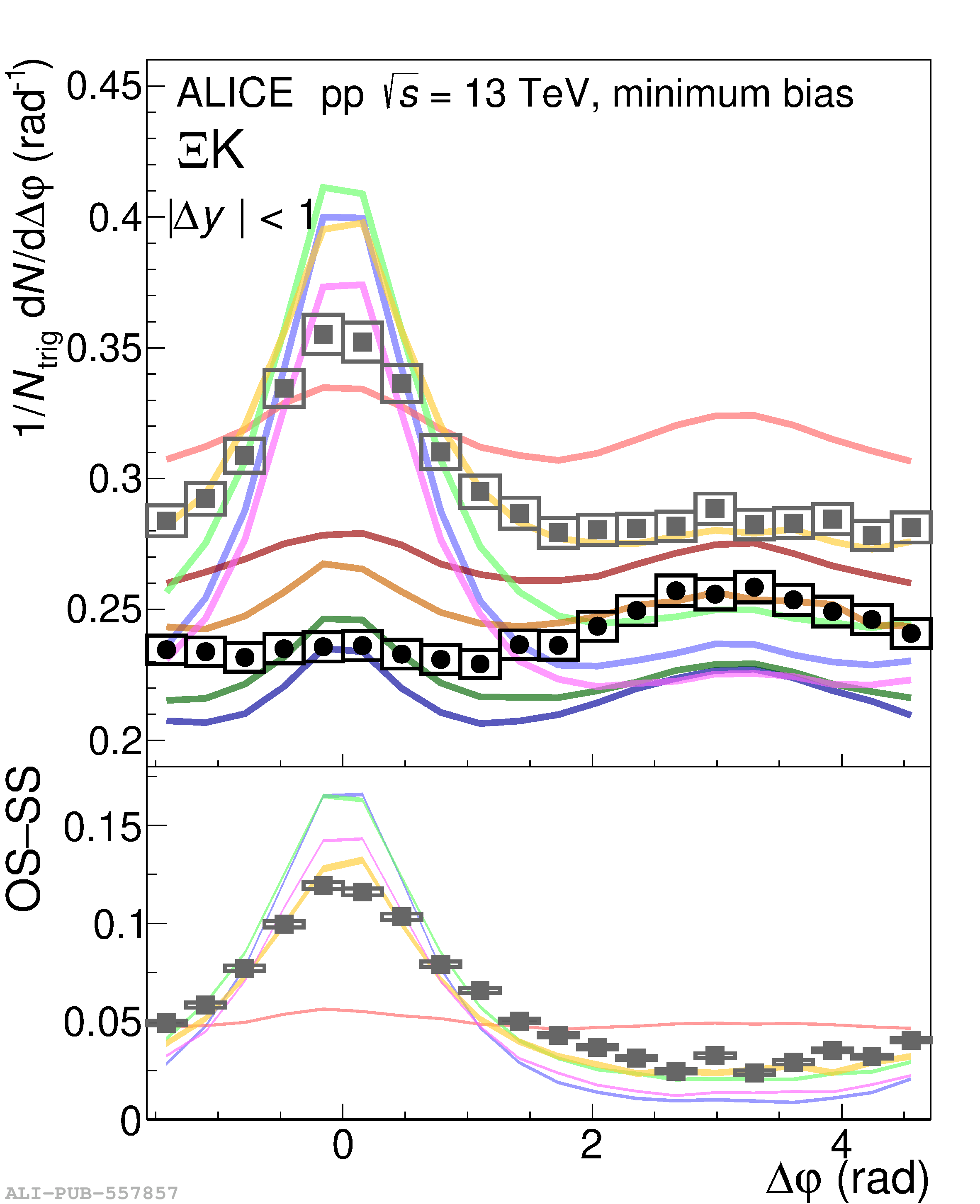 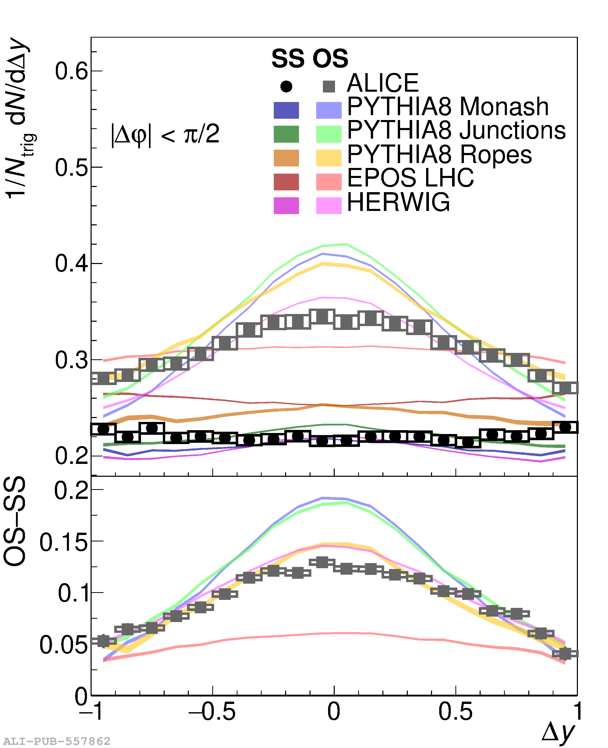 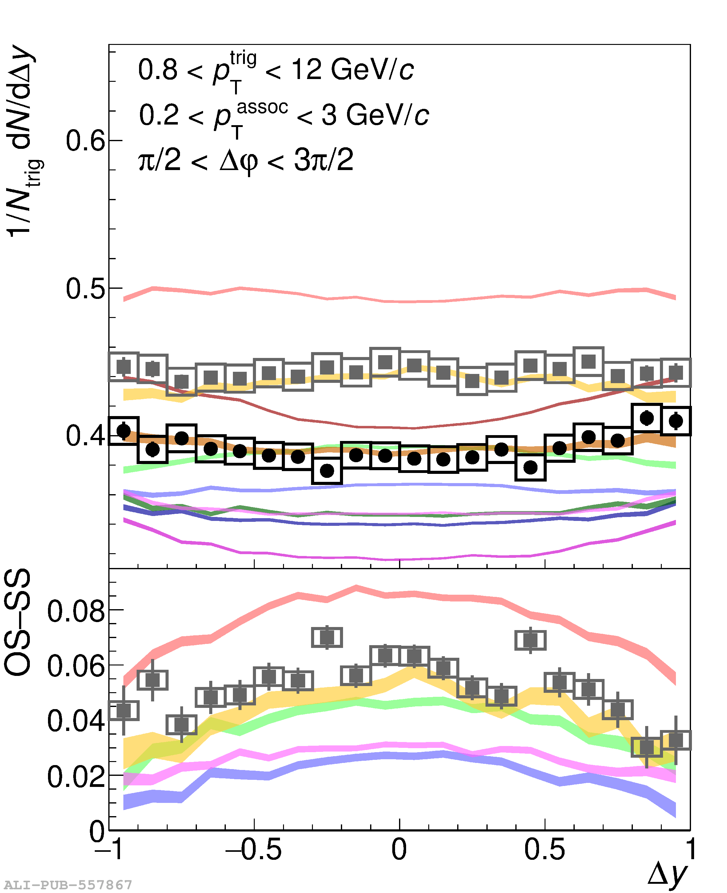 |
Figure 4
$\Xi\mathrm{p}$ (top row), $\Xi\Lambda$ (middle row), and $\Xi\Xi$ (bottom row) per-trigger yields in $(\Delta y,\Delta\varphi)$ for particle pair combinations with the opposite (left column) and same (right column) baryon number, measured in pp collisions at $\sqrt{s} = 13$ TeV. | 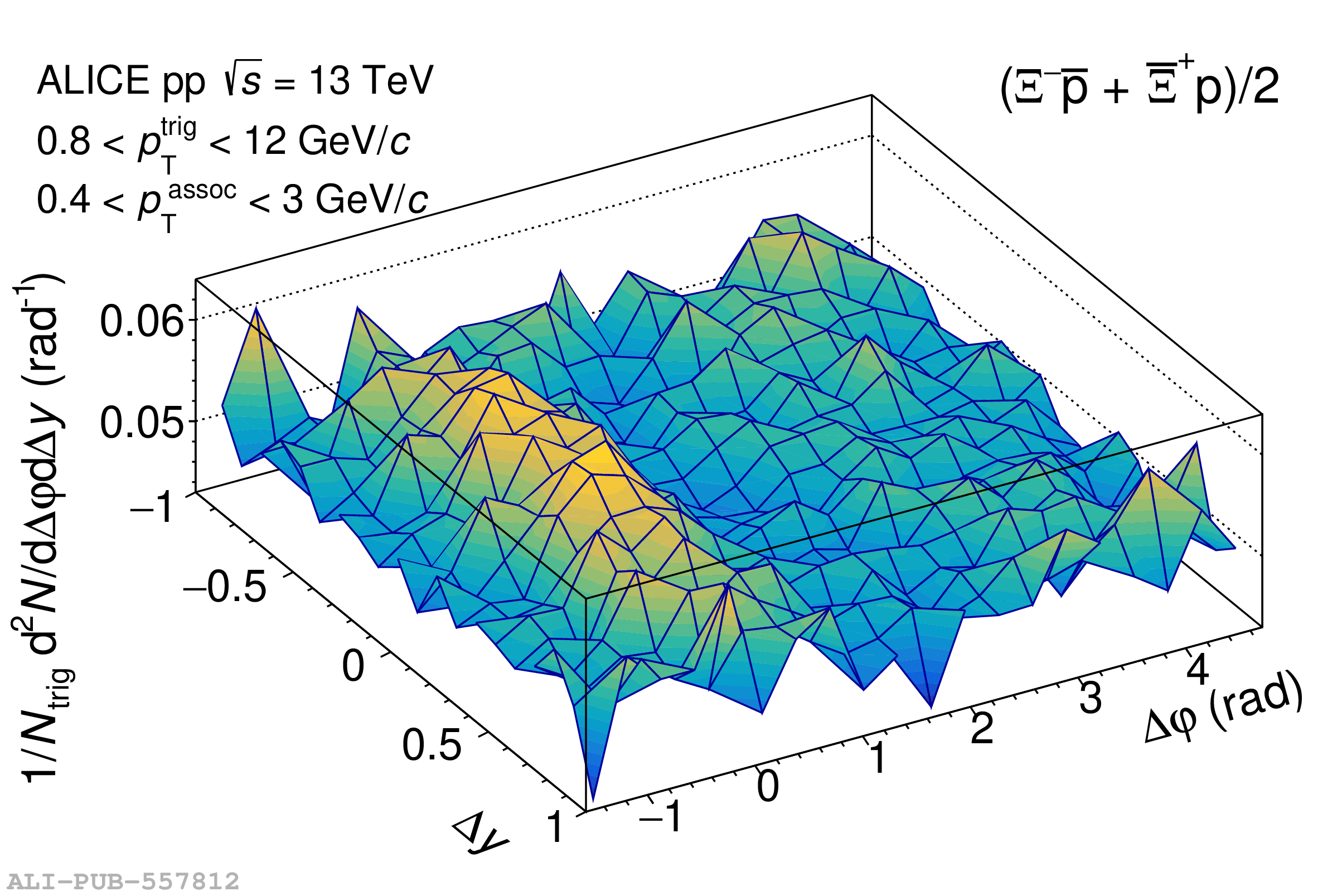 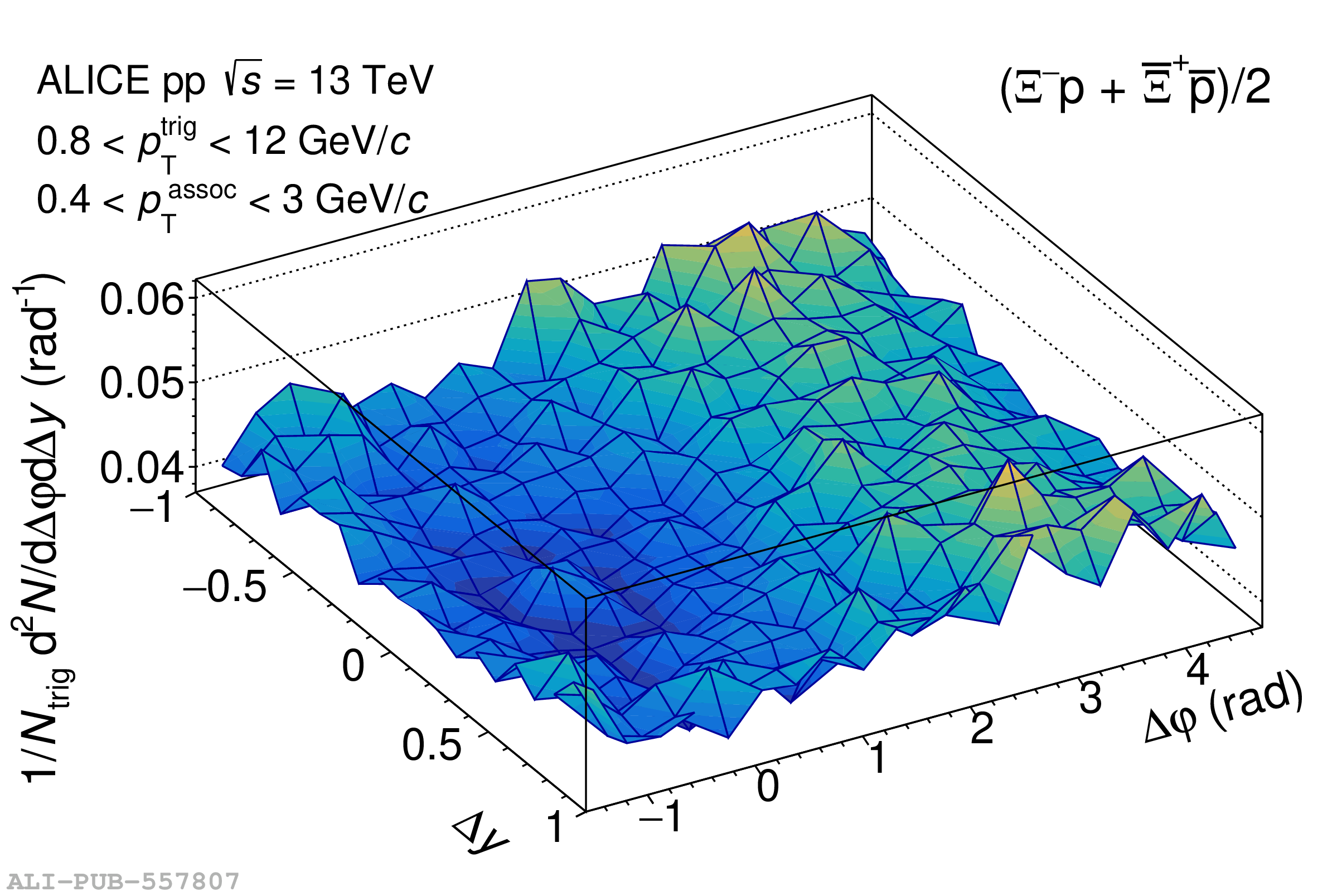 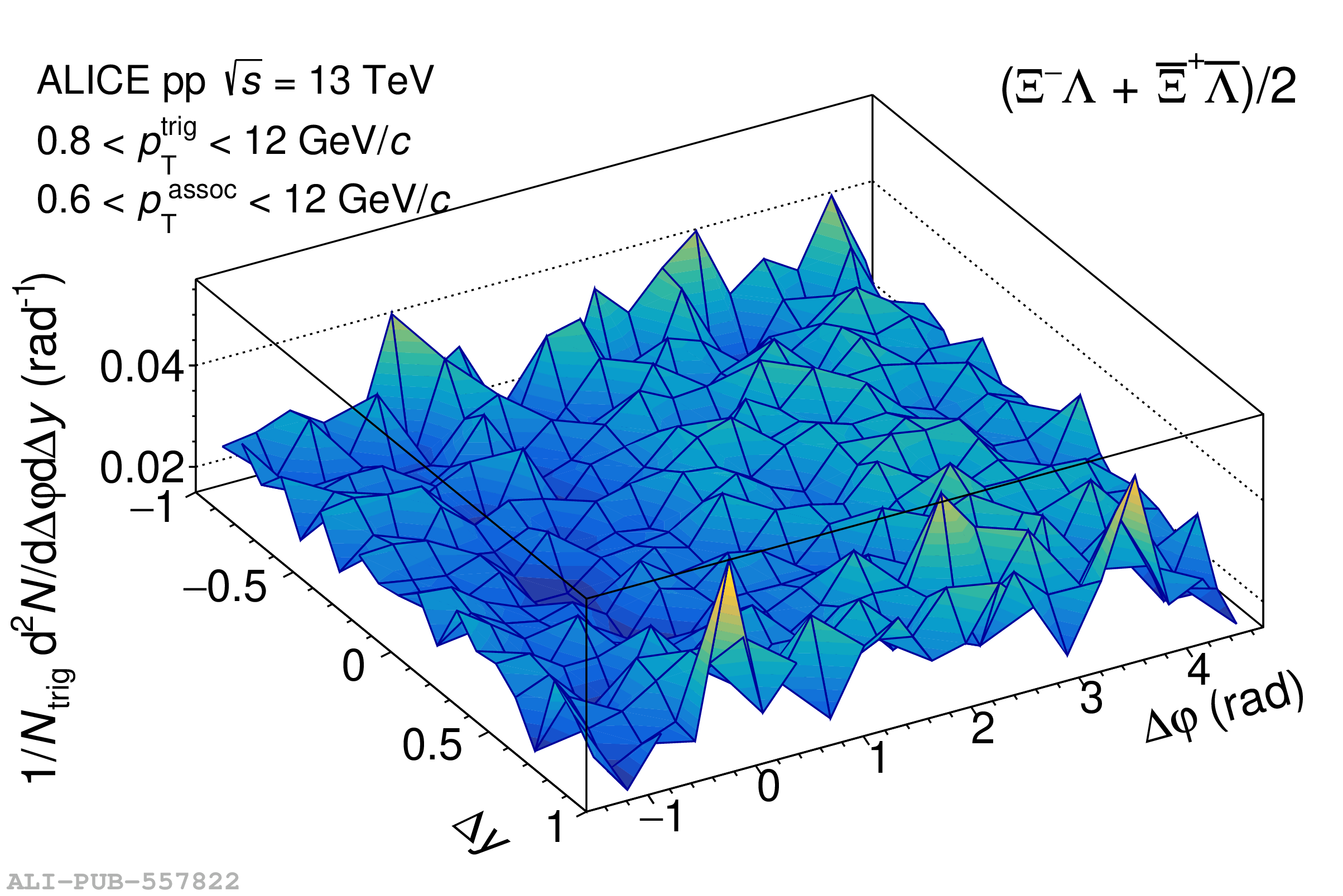 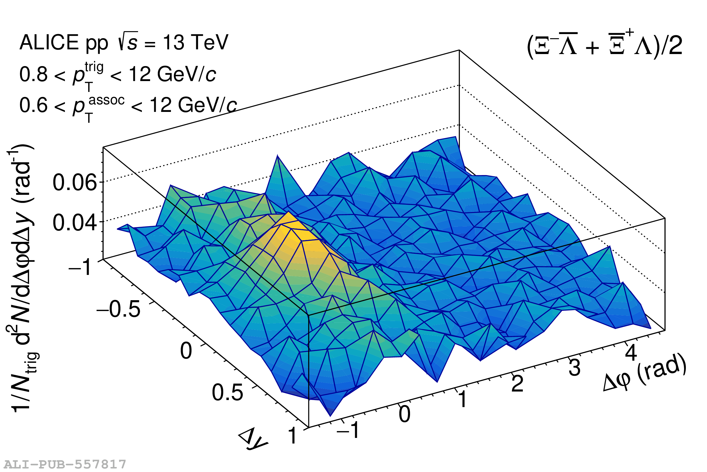 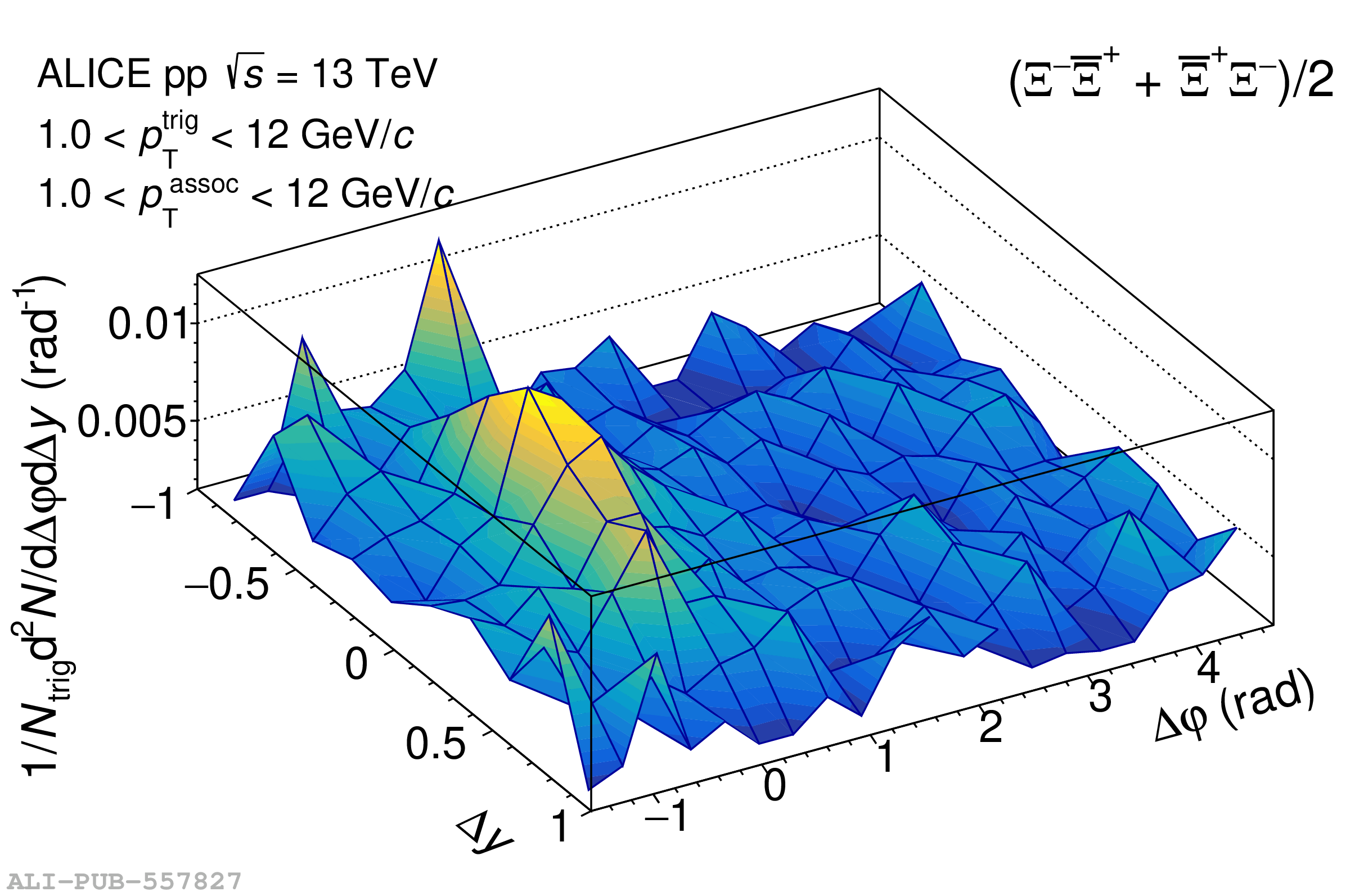 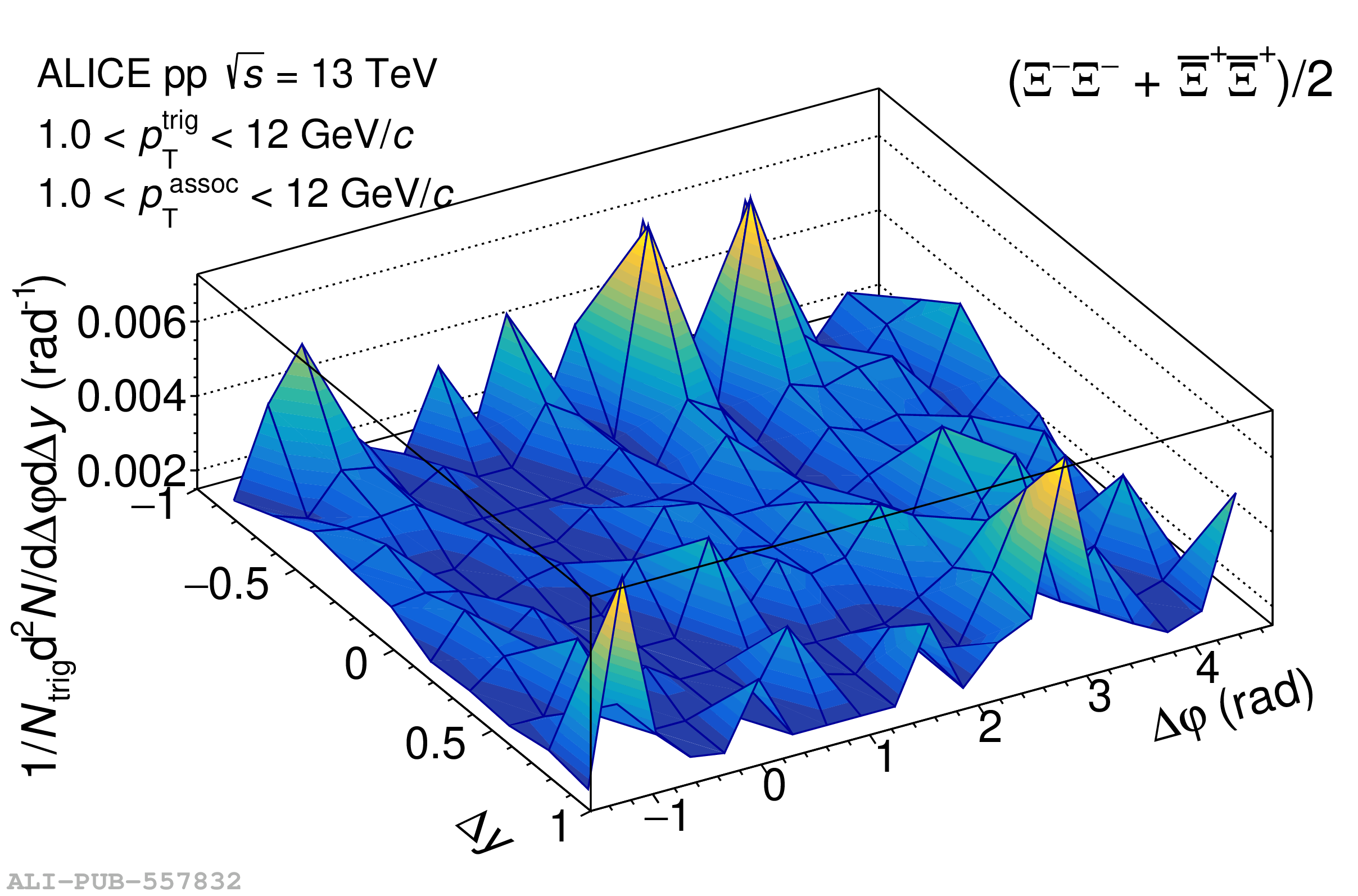 |
Figure 5
$\Xi^-\overline{\mathrm{p}}$ and $\Xi^-\mathrm{p}$ (and charge conjugate) correlation functions projected onto $\Delta\varphi$ ($|\Delta y| < 1$, left), the near-side on $\Delta y$ ($|\Delta\varphi| < \pi/2$, middle), and the away-side on $\Delta y$ ($\pi/2 < \Delta\varphi < 3\pi/2$, right). Opposite-baryon-number ($\Xi^{-}\overline{\mathrm{p}}+\overline{\Xi}^{+}\mathrm{p}$) correlations are shown in grey squares, the same-baryon-number ($\Xi^{-}\mathrm{p}+\overline{\Xi}^{+}\overline{\mathrm{p}}$) correlations are black circles; the OB$-$SB difference is displayed in the bottom panels. Statistical and systematic uncertainties are represented by bars and boxes, respectively. The ALICE data are compared with the following models: PYTHIA 8 Monash tune (blue), PYTHIA 8 with junctions enabled (green), PYTHIA 8 with junctions and ropes (yellow), EPOS-LHC (red), and HERWIG 7 (pink). | 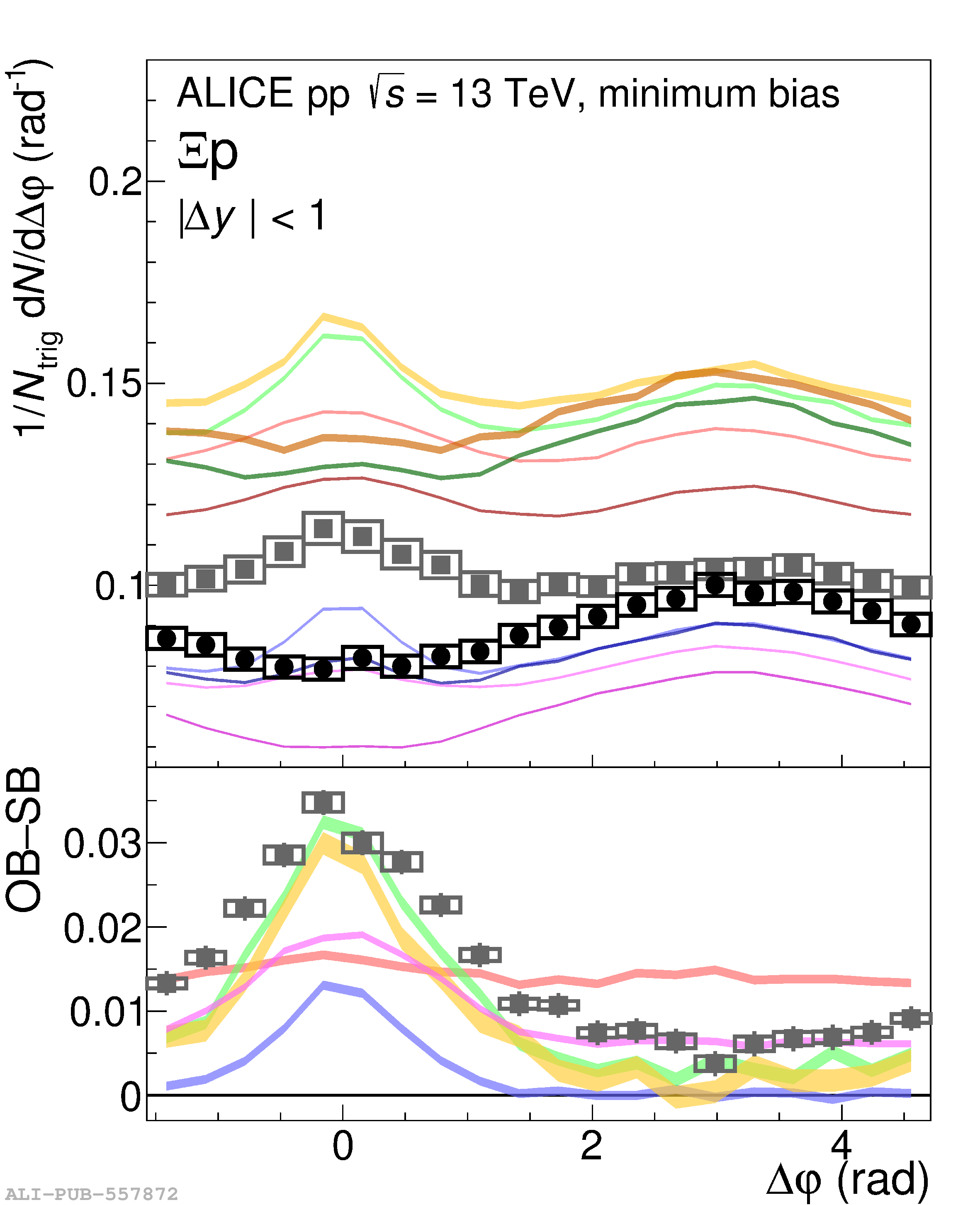 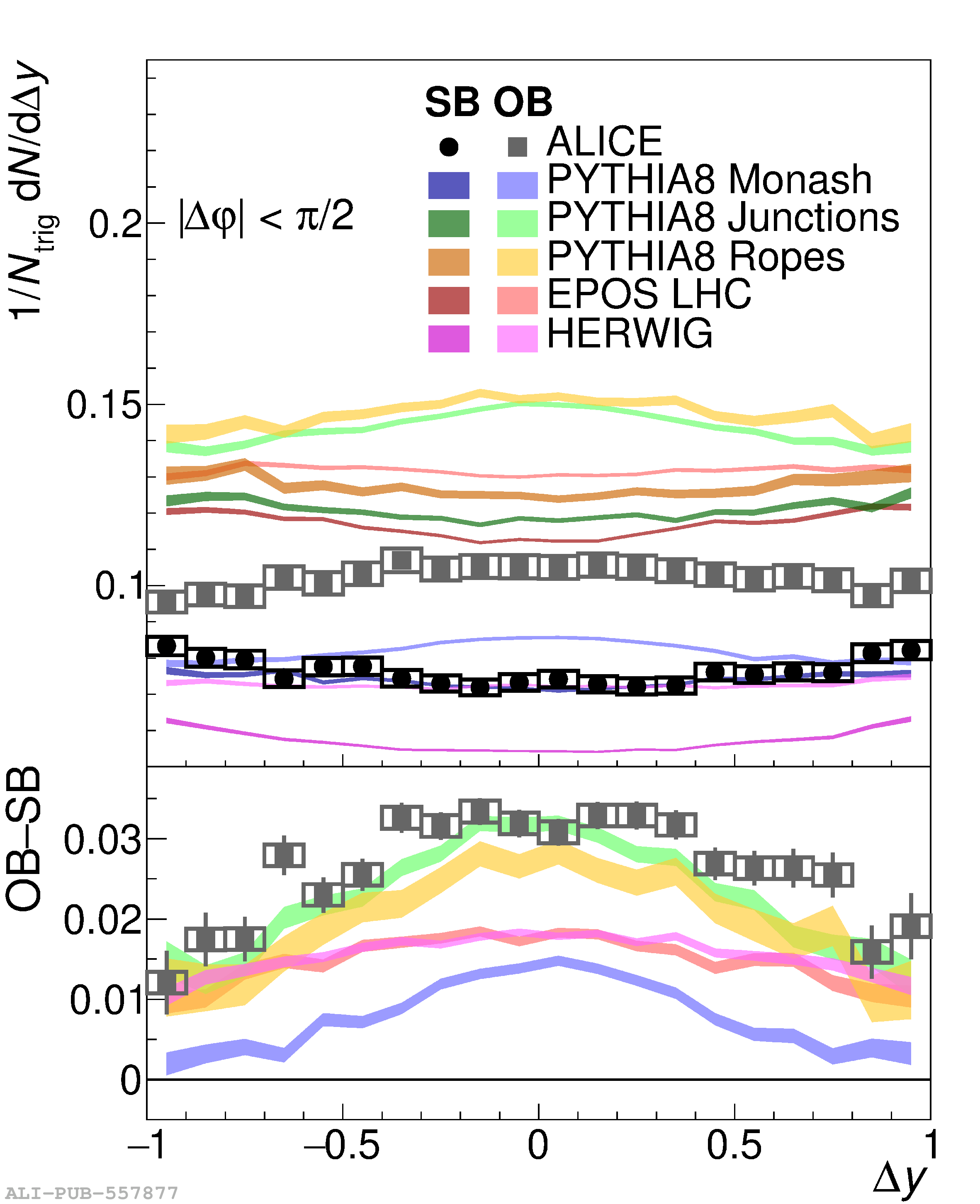 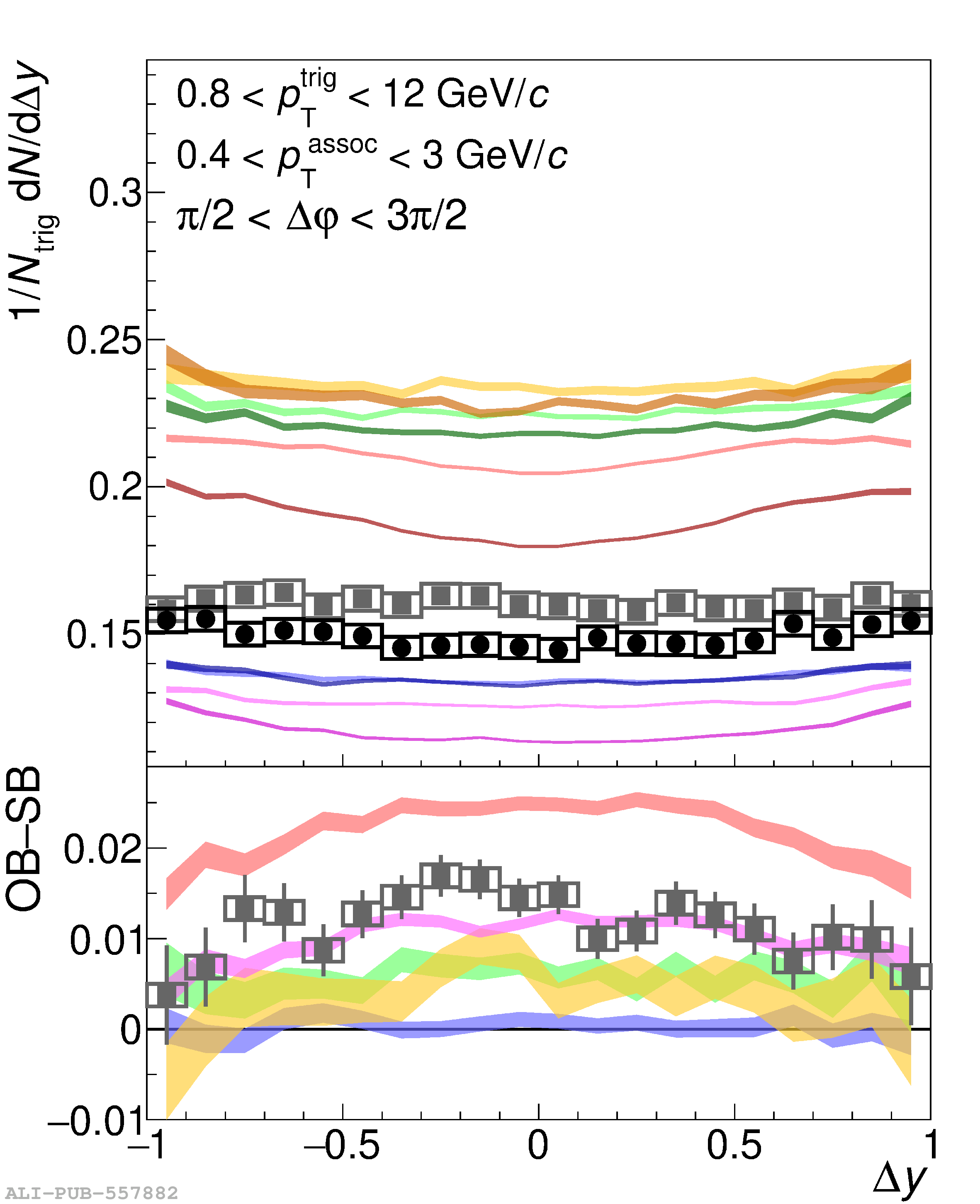 |
Figure 6
$\Xi^-\overline{\Lambda}$ and $\Xi^-\Lambda$ (and charge conjugate) correlation functions projected onto $\Delta\varphi$ ($|\Delta y| < 1$, left), the near-side on $\Delta y$ ($|\Delta\varphi| < \pi/2$, middle), and the away-side on $\Delta y$ ($\pi/2 < \Delta\varphi < 3\pi/2$, right). Opposite-baryon-number ($\Xi^{-}\overline{\Lambda}+\overline{\Xi}^{+}\Lambda$) correlations are shown in grey squares, the same-baryon-number ($\Xi^{-}\Lambda+\overline{\Xi}^{+}\overline{\Lambda}$) correlations are black circles; the OB$-$SB difference is displayed in the bottom panels. Statistical and systematic uncertainties are represented by bars and boxes, respectively. The ALICE data are compared with the following models: PYTHIA 8 Monash tune (blue), PYTHIA 8 with junctions enabled (green), PYTHIA 8 with junctions and ropes (yellow), EPOS-LHC (red), and HERWIG 7 (pink). | 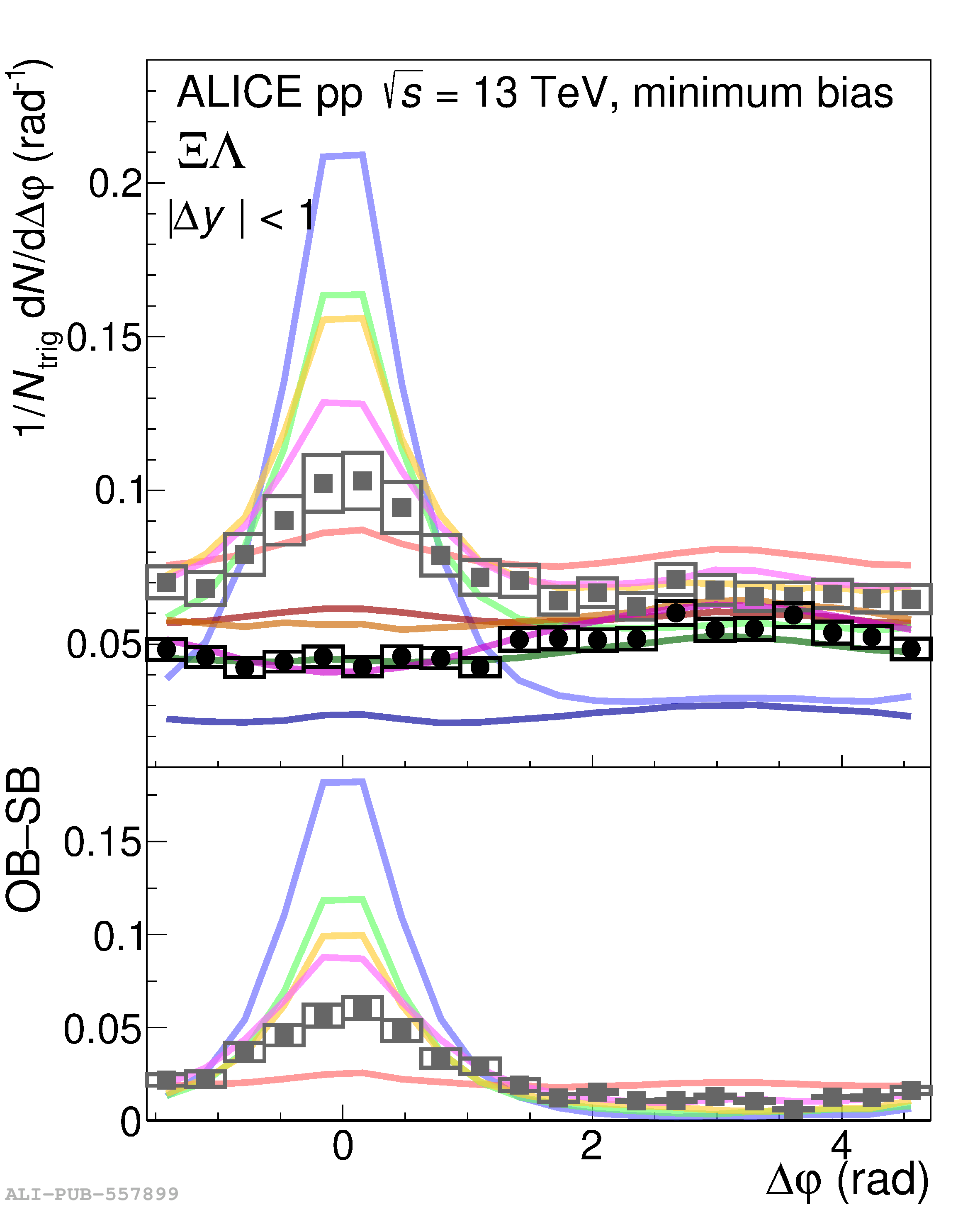 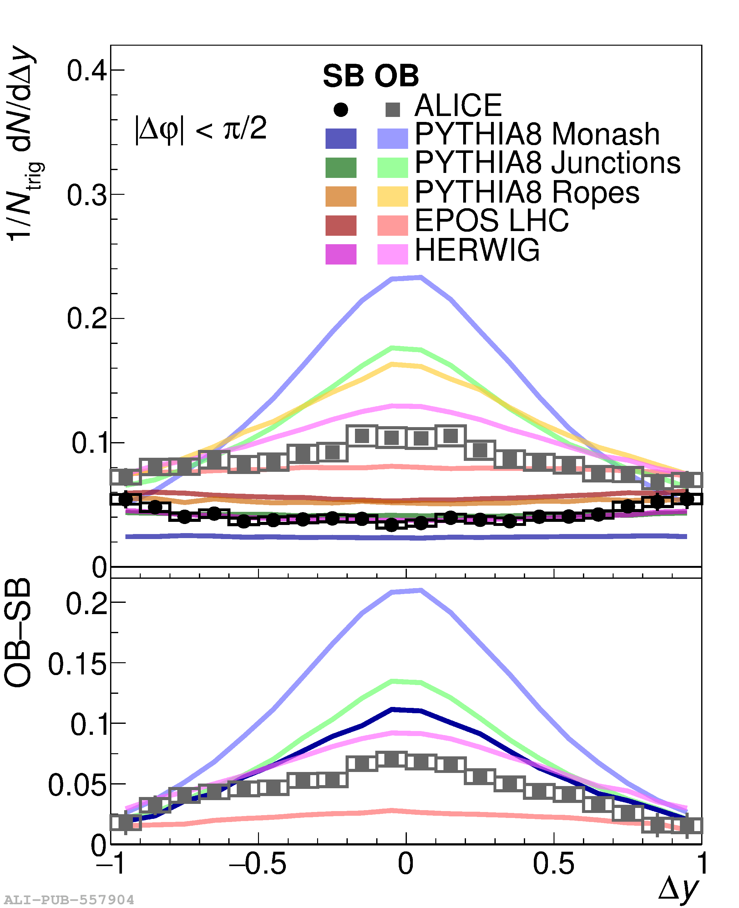 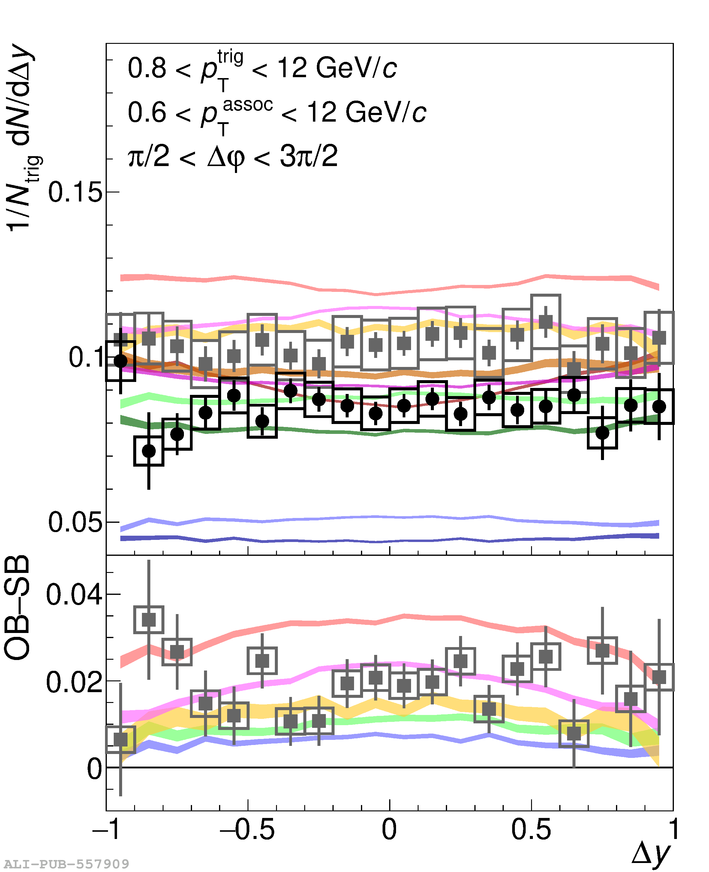 |
Figure 7
$\Xi^-\overline{\Xi}^+$ and $\Xi^-\Xi^-$ (and charge conjugate) correlation functions projected onto $\Delta\varphi$ ($|\Delta y| < 1$, left), the near-side on $\Delta y$ ($|\Delta\varphi| < \pi/2$, middle), and the away-side on $\Delta y$ ($\pi/2 < \Delta\varphi < 3\pi/2$, right). Opposite-baryon-number ($\Xi^{-}\overline{\Xi}^{+}+\overline{\Xi}^{+}\Xi^{-}$) correlations are shown in grey squares, the same-baryon-number ($\Xi^{-}\Xi^{-}+\overline{\Xi}^{+}\overline{\Xi}^{+}$) correlations are black circles; the OB$-$SB difference is displayed in the bottom panels. Statistical and systematic uncertainties are represented by bars and boxes, respectively. The ALICE data are compared with the following models: PYTHIA 8 Monash tune (blue), PYTHIA 8 with junctions enabled (green), PYTHIA 8 with junctions and ropes (yellow), EPOS-LHC (red), and HERWIG 7 (pink). | 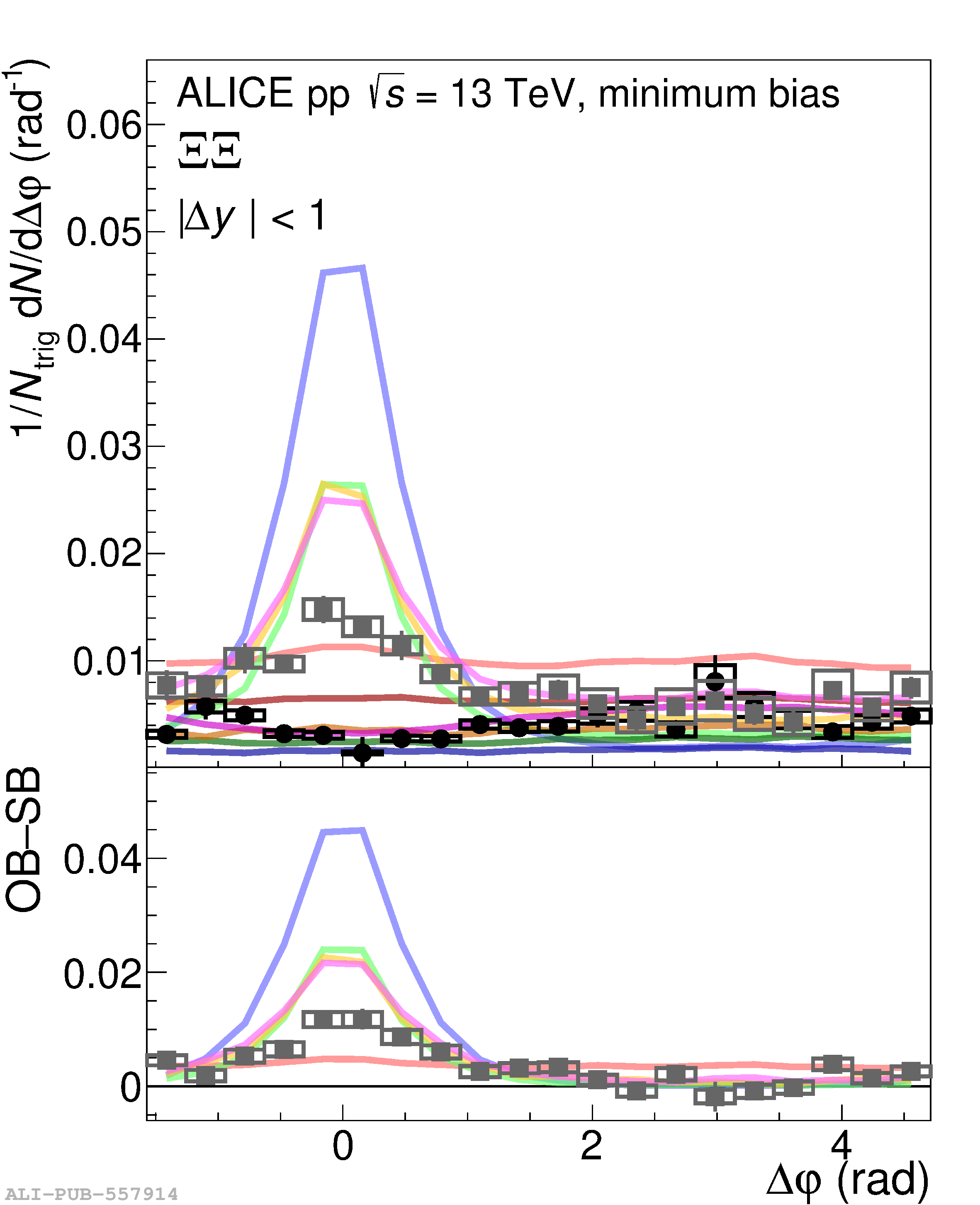 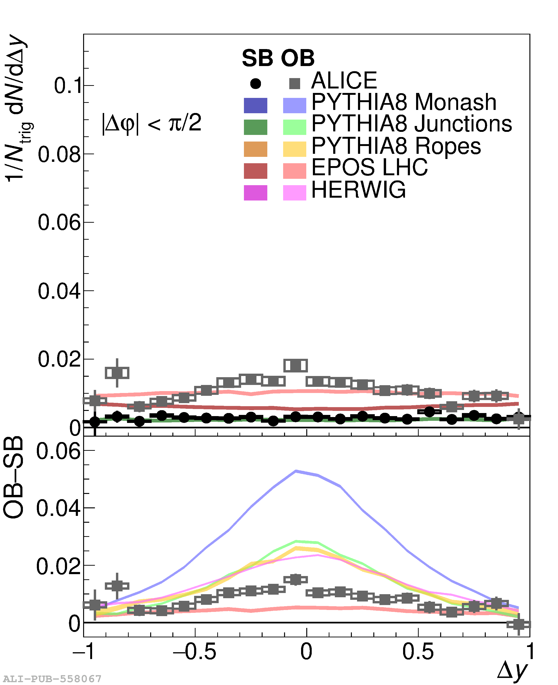 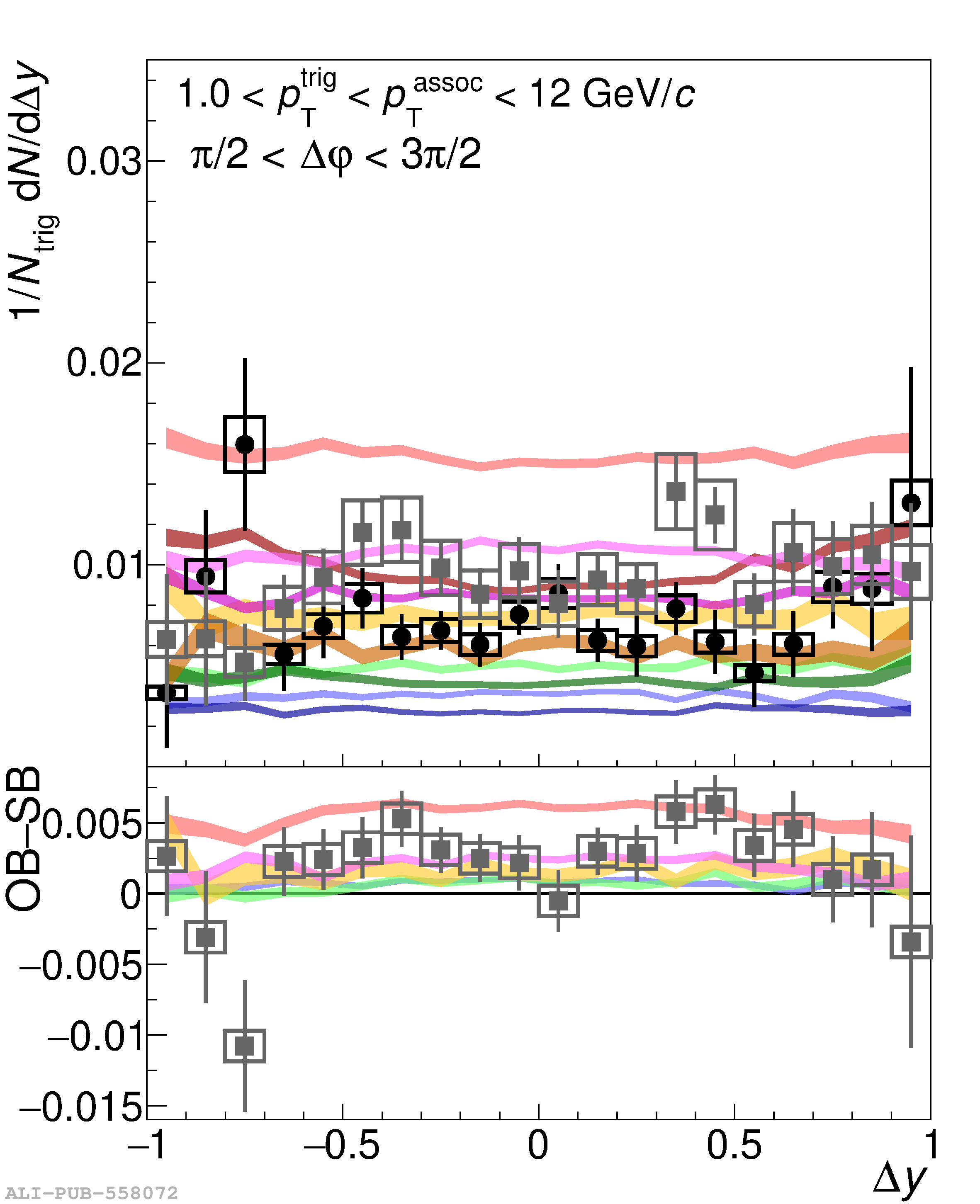 |
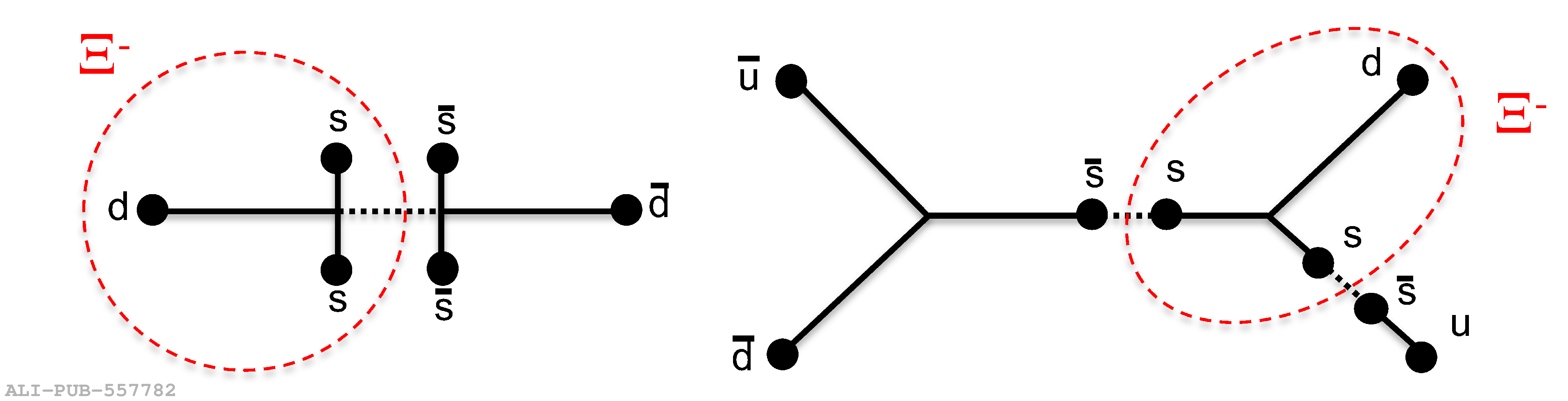
Figure 9
The OS$-$SS and OB$-$SB per-trigger yields for $\Xi\pi$, $\Xi\mathrm{K}$, $\Xi\mathrm{p}$, $\Xi\Lambda$, and $\Xi\Xi$ correlations are shown when integrated over all phase space (top), on the near-side ($|\Delta\varphi| < \pi/2$, bottom left), and on the away-side ($\pi/2 < \Delta\varphi < 3\pi/2$, bottom right). Statistical and systematic uncertainties are represented by bars and boxes, respectively. The ALICE data are compared with the following models: PYTHIA 8 Monash tune (blue), PYTHIA 8 with junctions enabled (green), PYTHIA 8 with junctions and ropes (yellow), EPOS-LHC (red), and HERWIG 7 (pink). The statistical uncertainties on the model predictions are smaller than the marker sizes. | 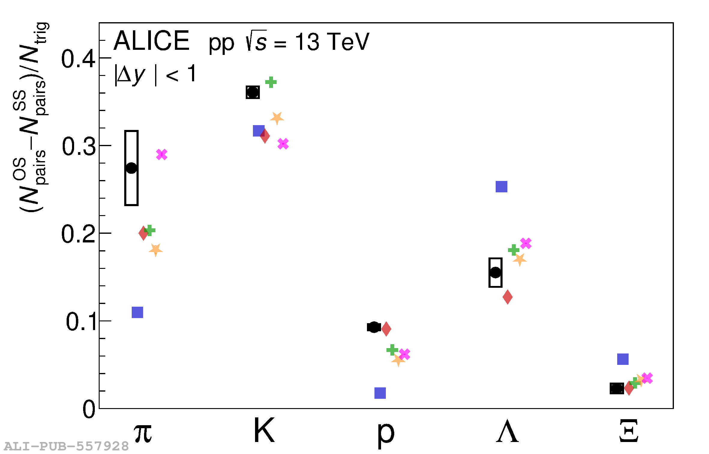 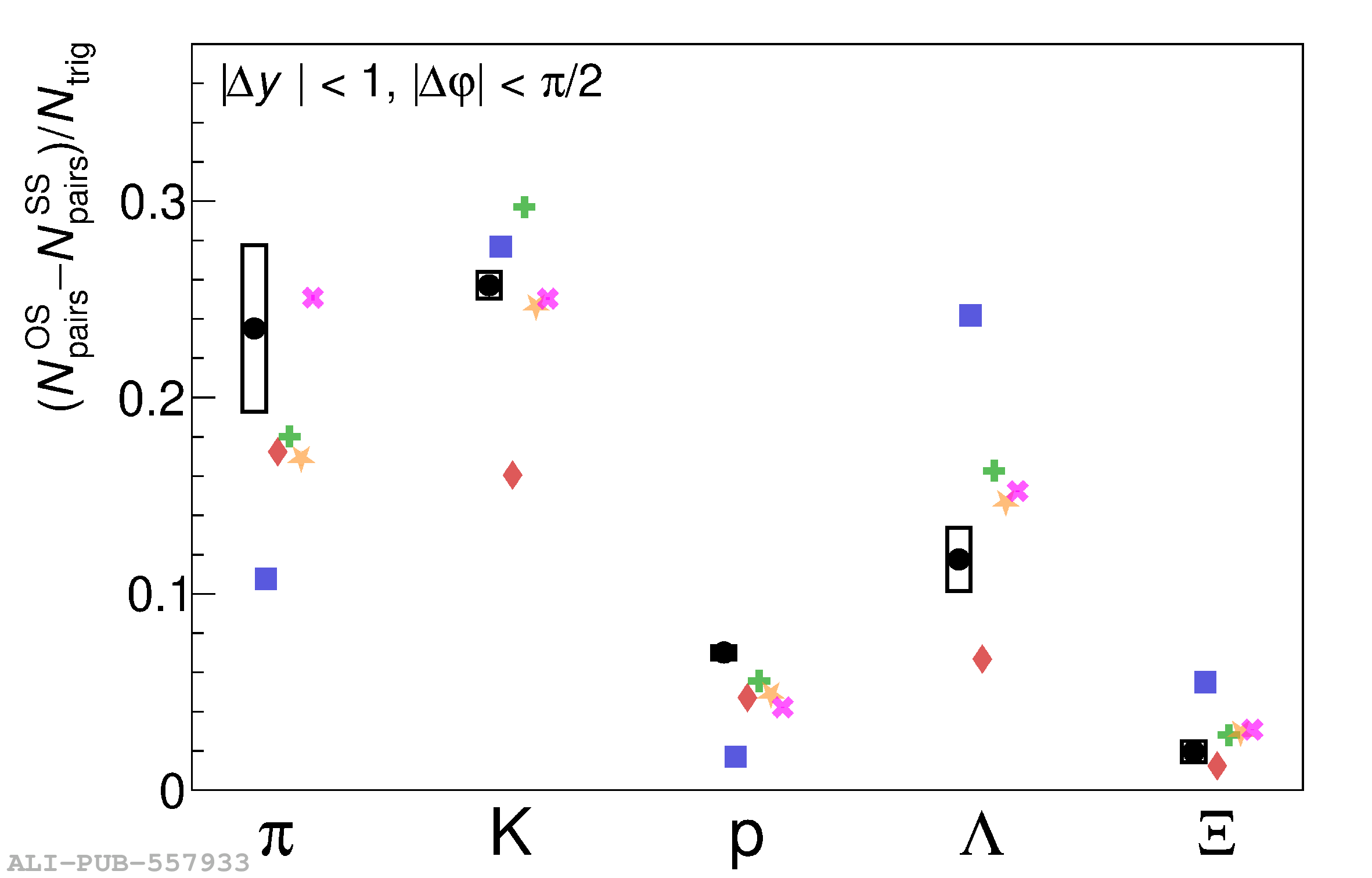 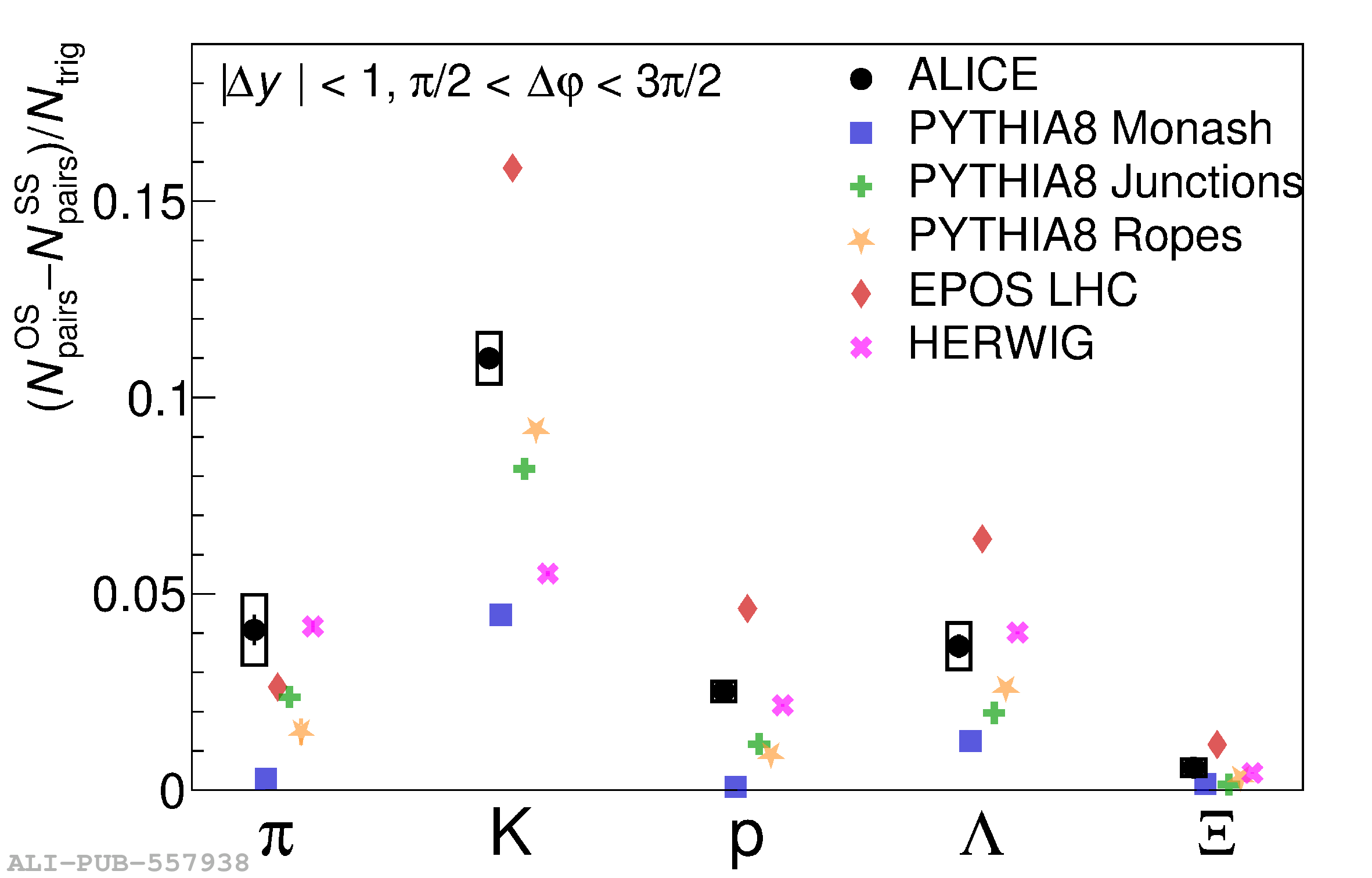 |
Figure 10
The $\Xi\pi$ (top left), $\Xi$K (top centre), $\Xi$p (bottom left), $\Xi\Lambda$ (bottom centre), and $\Xi\Xi$ (bottom right) correlation functions are shown for minimum bias (black), high-multiplicity ($0-5\%$, red), and low-multiplicity ($40-100\%$, blue) events, projected onto $\Delta\varphi$ ($|\Delta y| < 1$). In the top panels, opposite-sign correlations are shown in light markers, the same-sign correlations are shown with darker markers. In the bottom panels, the OS$-$SS or OB$-$SB difference is shown in each multiplicity interval. Statistical and systematic uncertainties are represented by bars and boxes, respectively. | 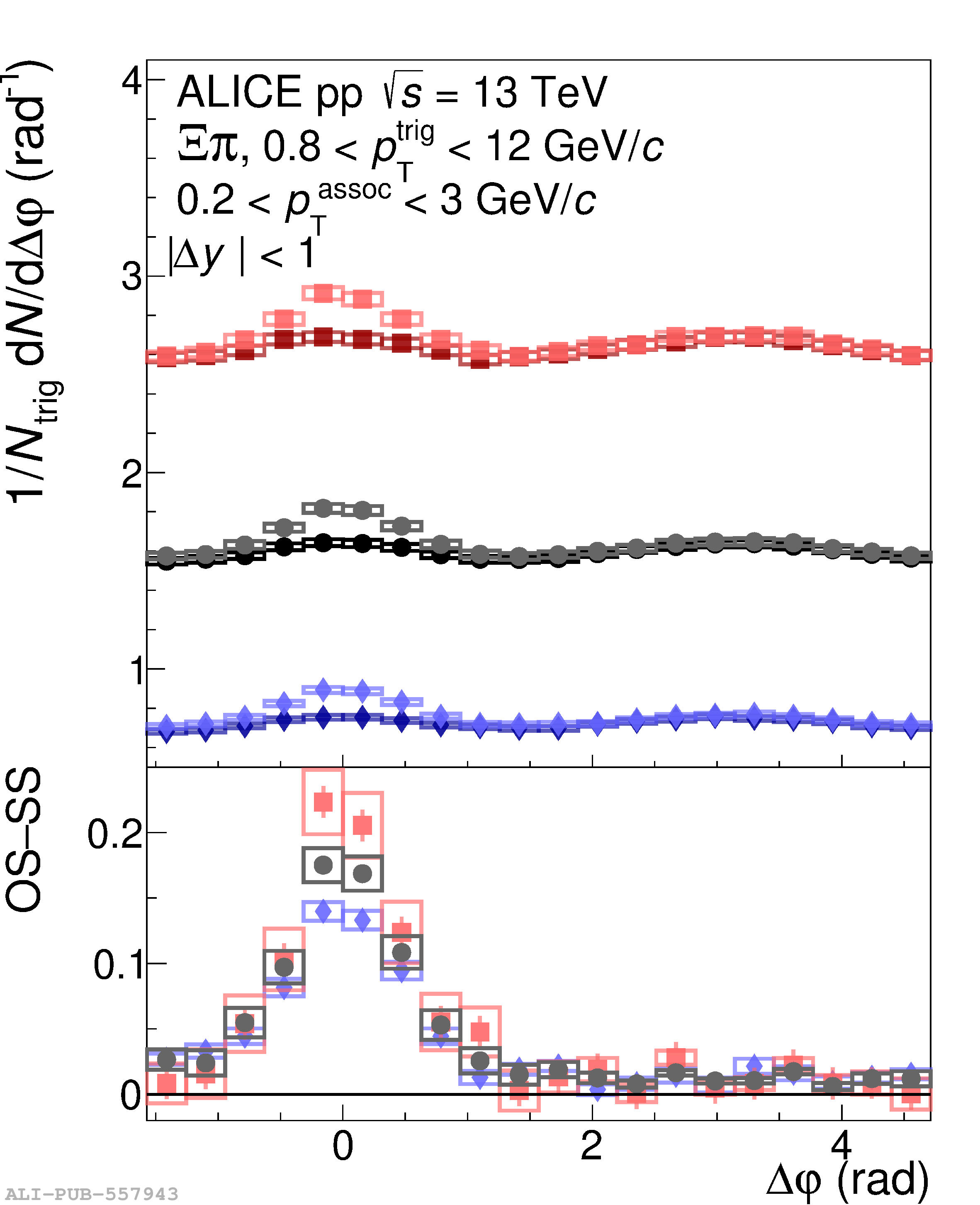 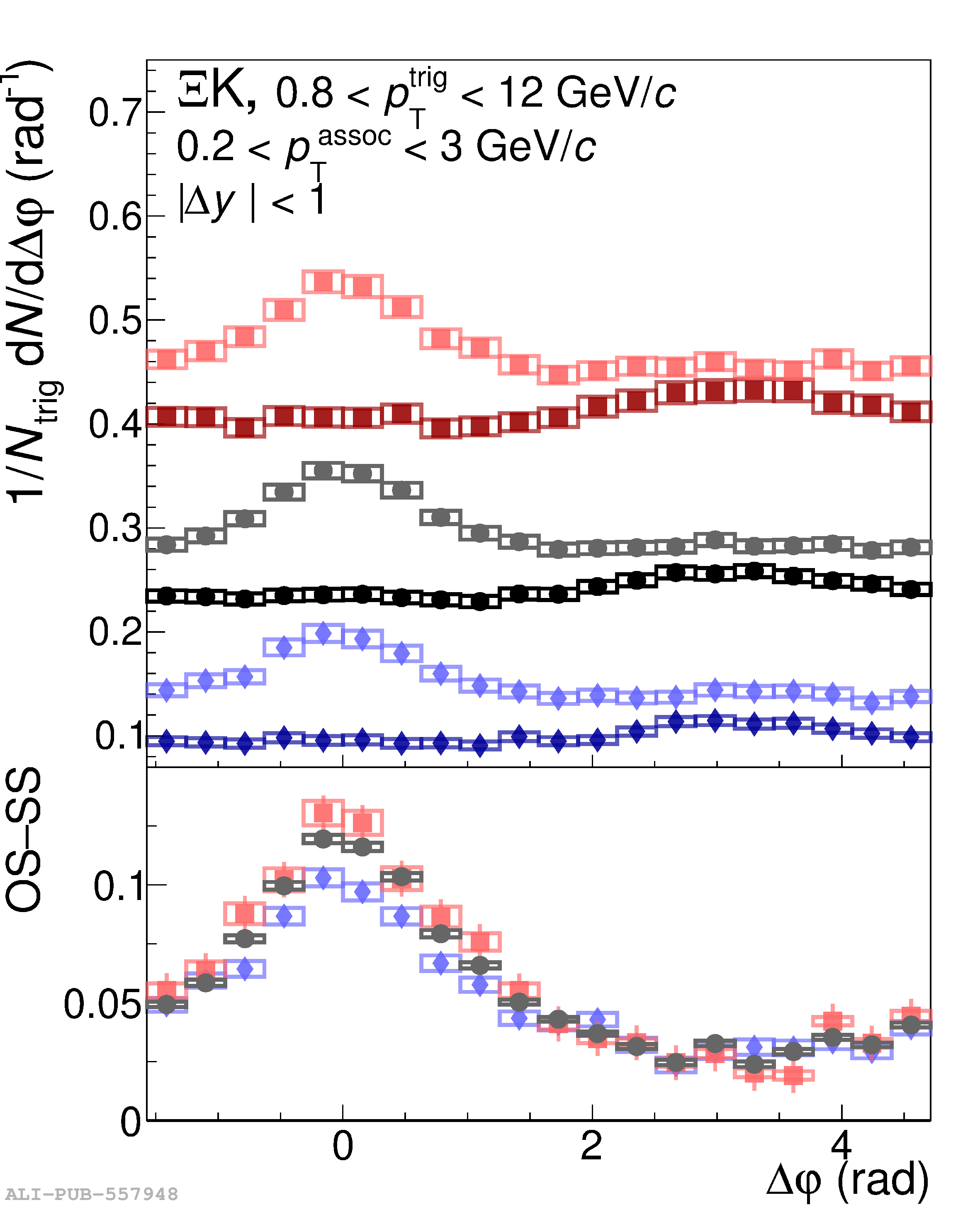  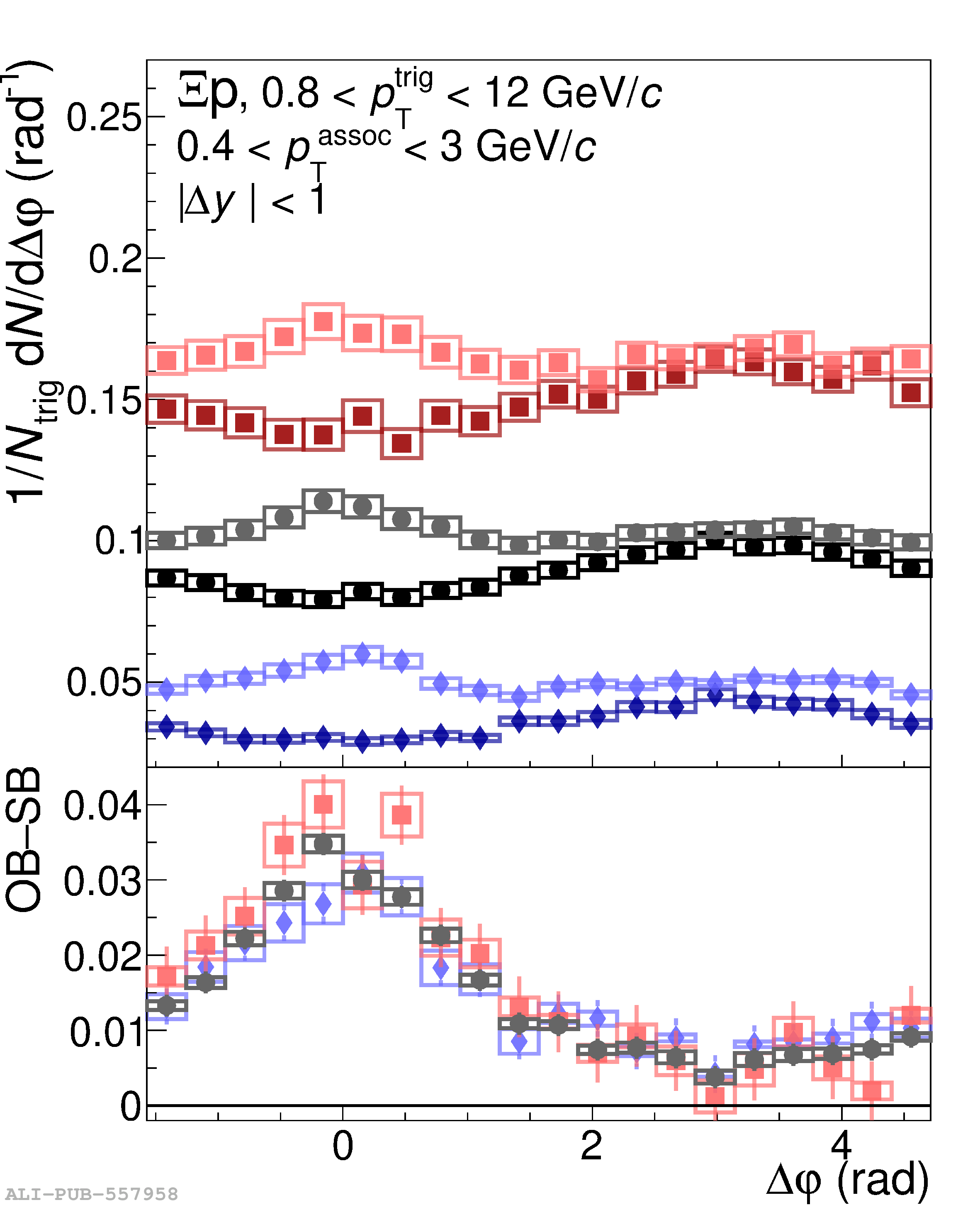 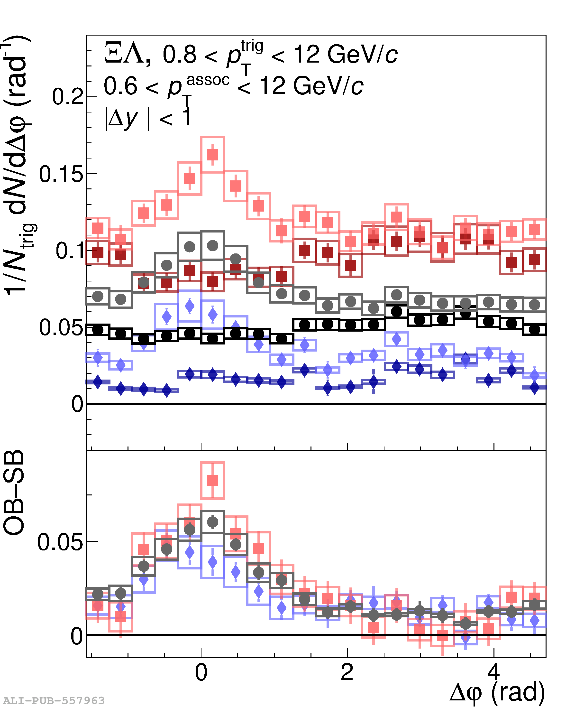 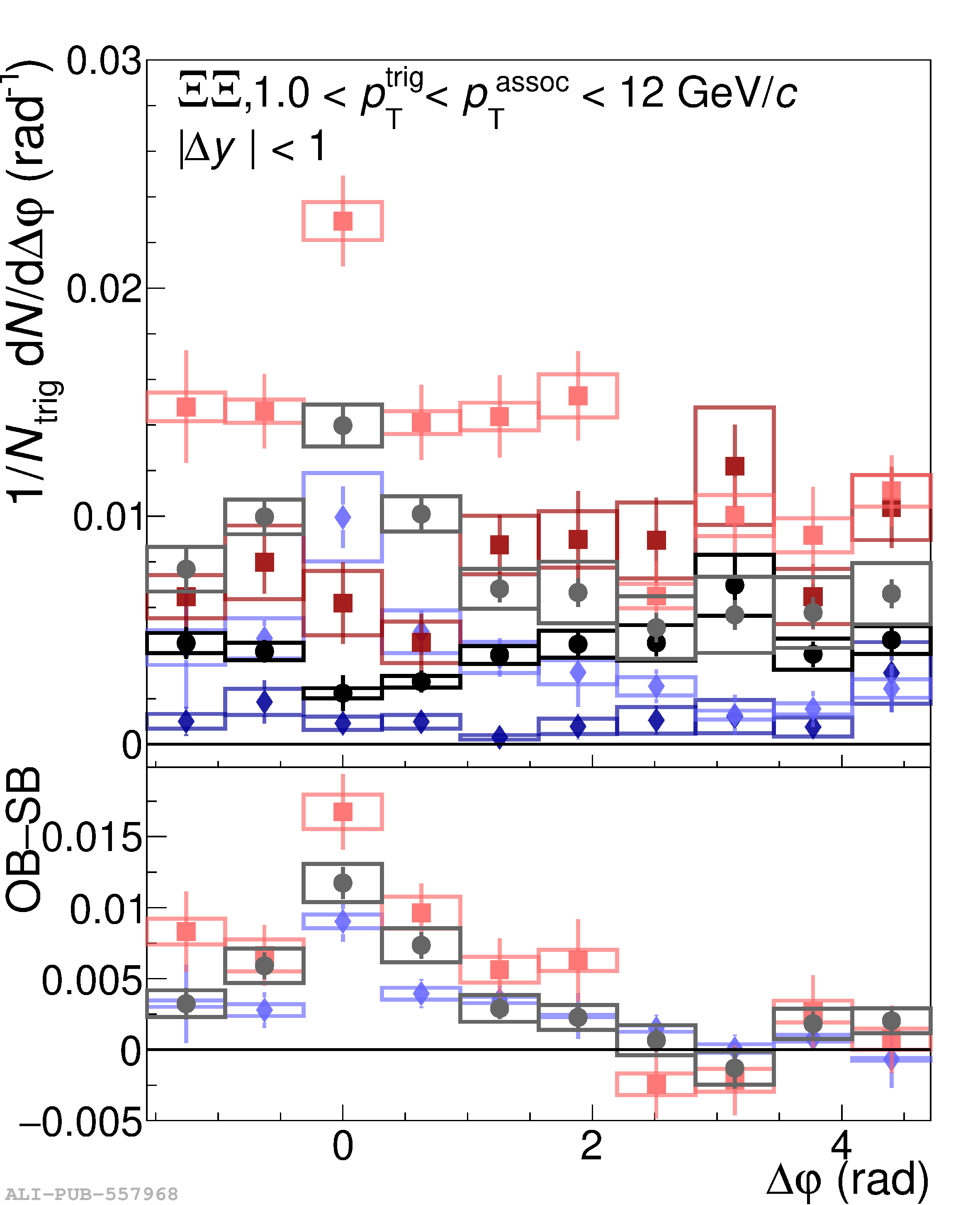 |
Figure 11
The $\Xi\pi$ (top left), $\Xi$K (top centre), $\Xi$p (bottom left), $\Xi\Lambda$ (bottom centre), and $\Xi\Xi$ (bottom right) correlation functions are shown for minimum bias (black), high-multiplicity ($0-5\%$, red), and low-multiplicity ($40-100\%$, blue) events, projected onto $\Delta y$ on the near side ($|\Delta\varphi| < \pi/2$). In the top panels, opposite-sign correlations are shown in light markers, the same-sign correlations are shown with darker markers. In the bottom panels, the OS$-$SS or OB$-$SB difference is shown in each multiplicity interval. Statistical and systematic uncertainties are represented by bars and boxes, respectively. | 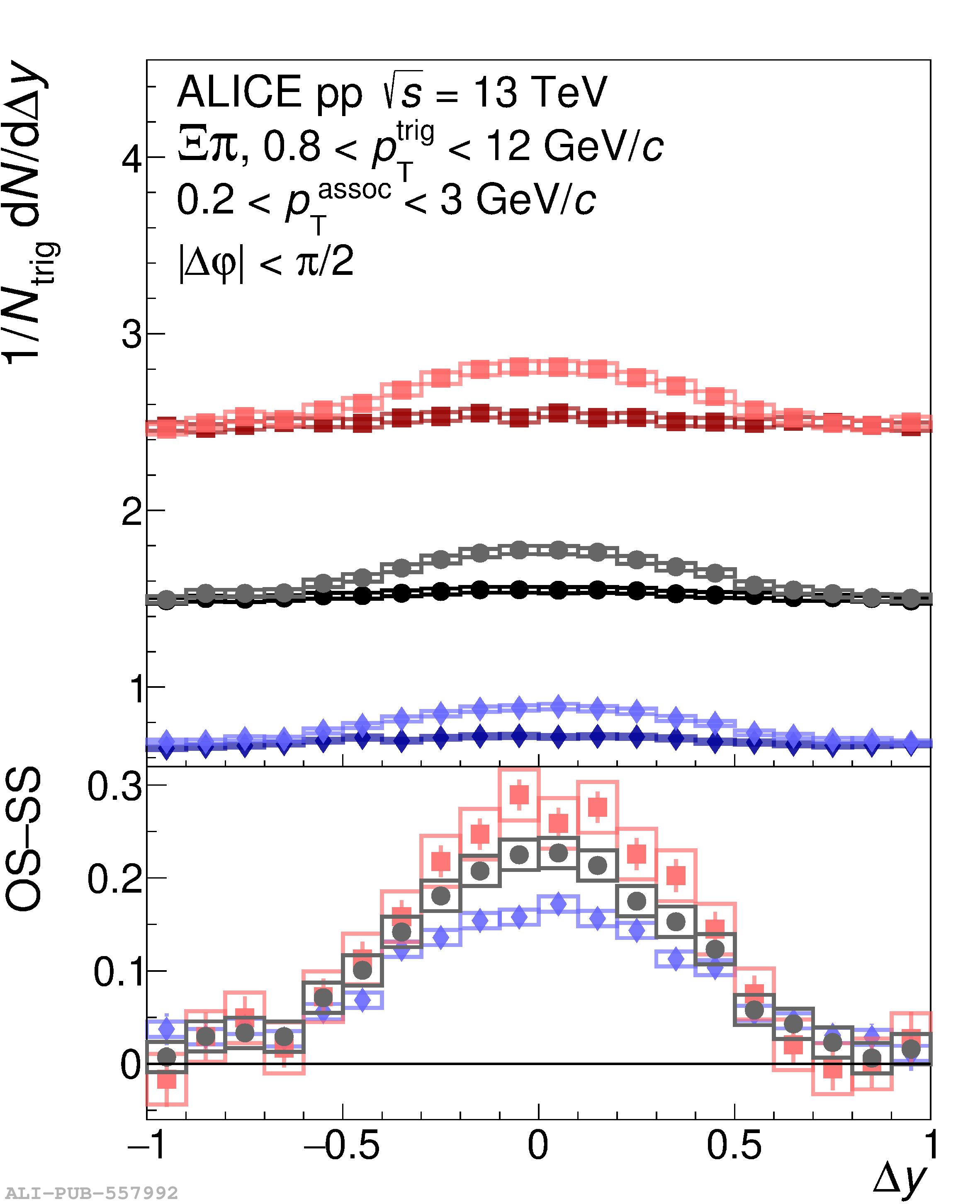 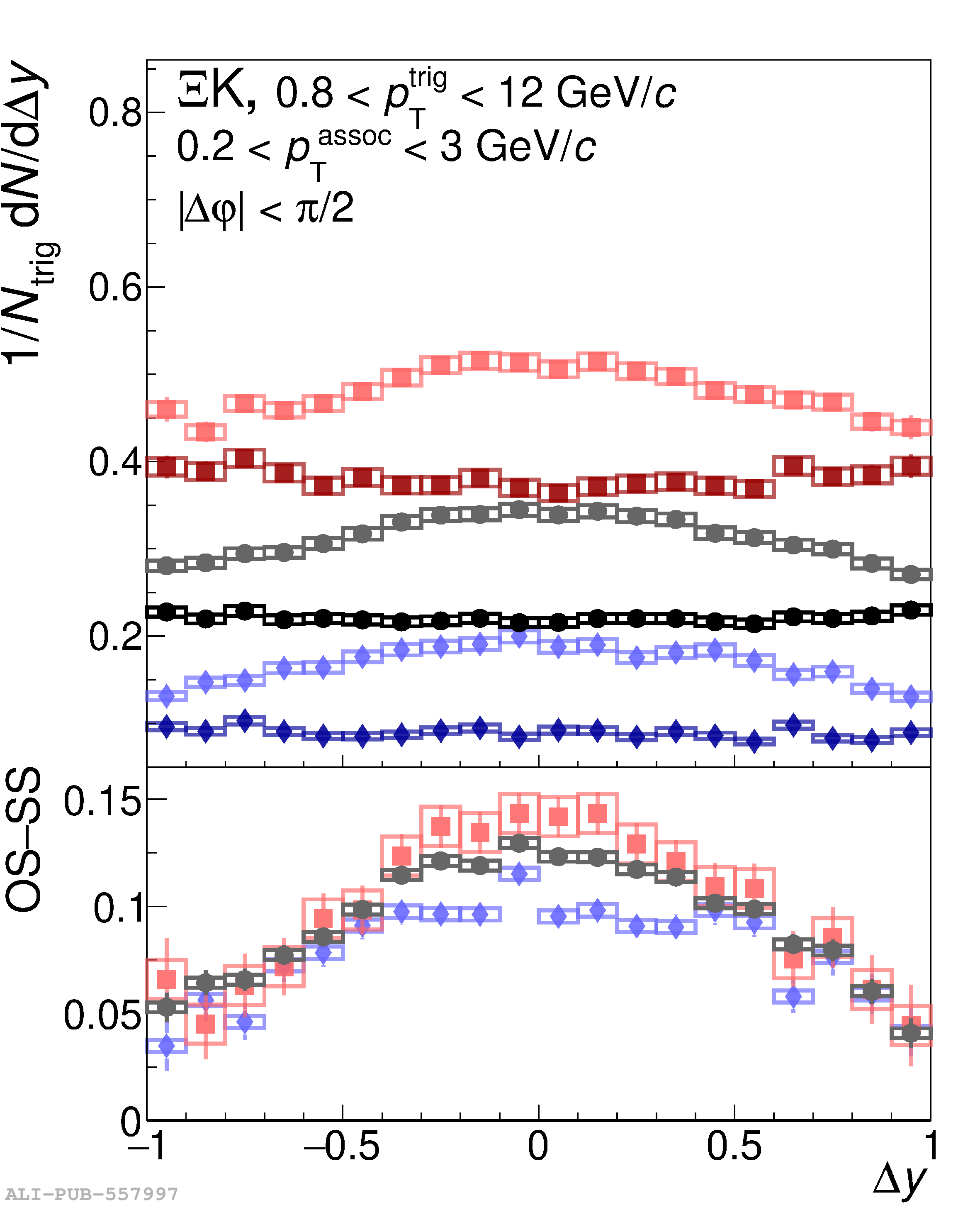 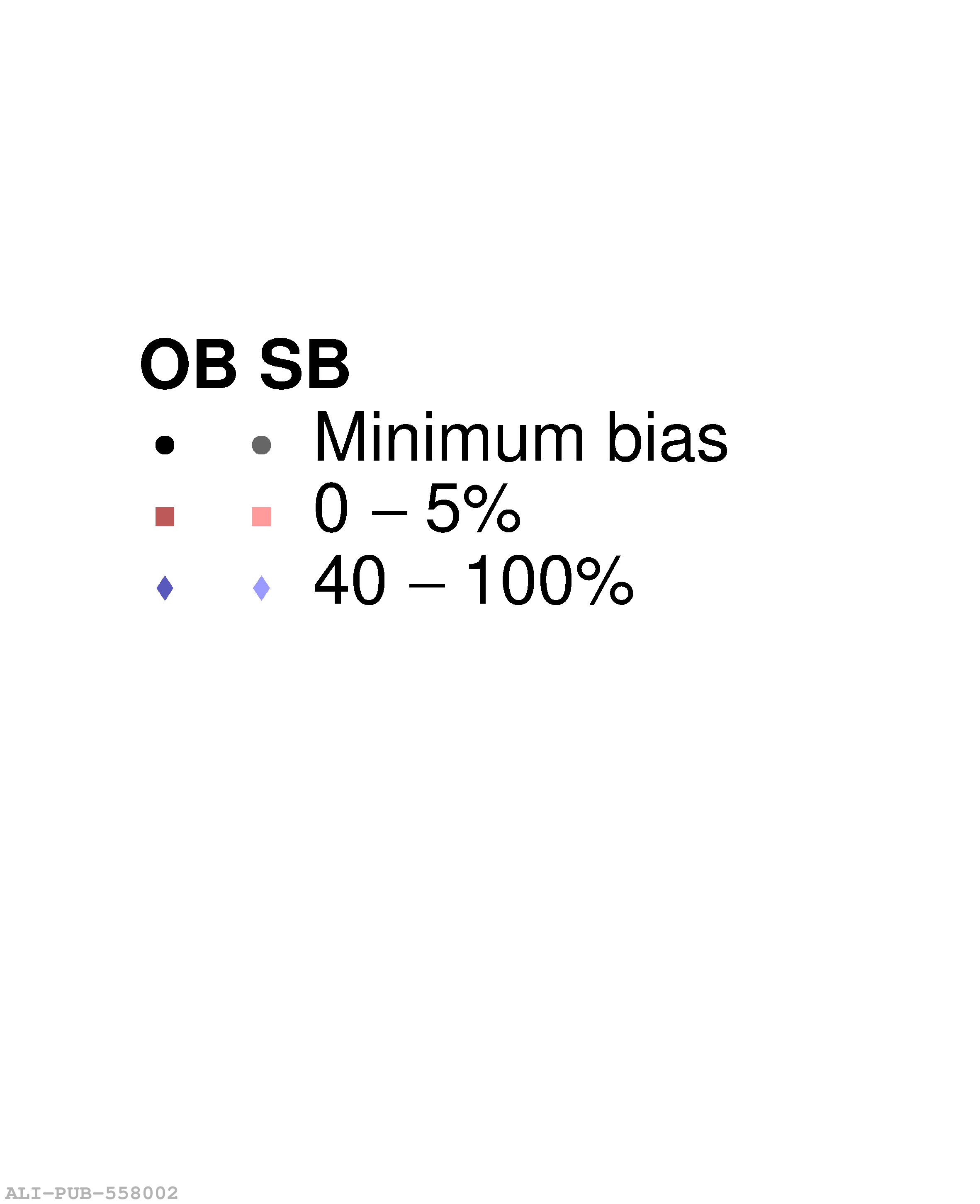 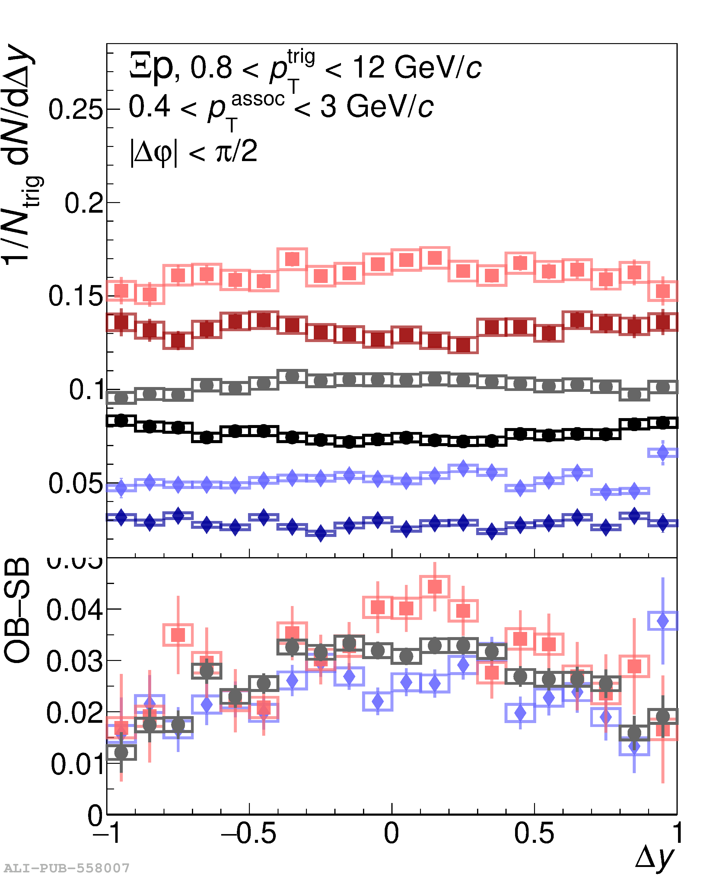 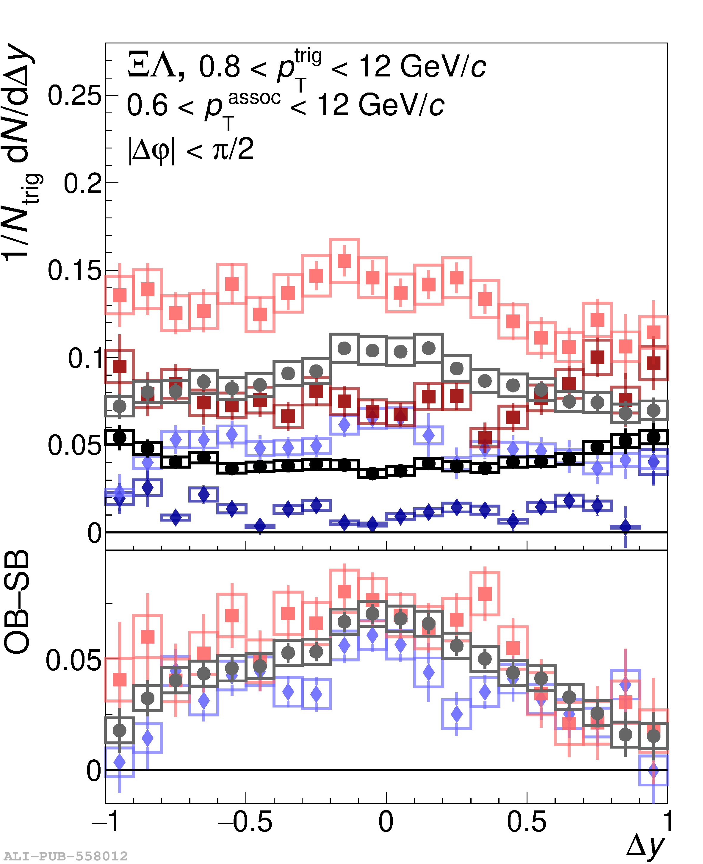 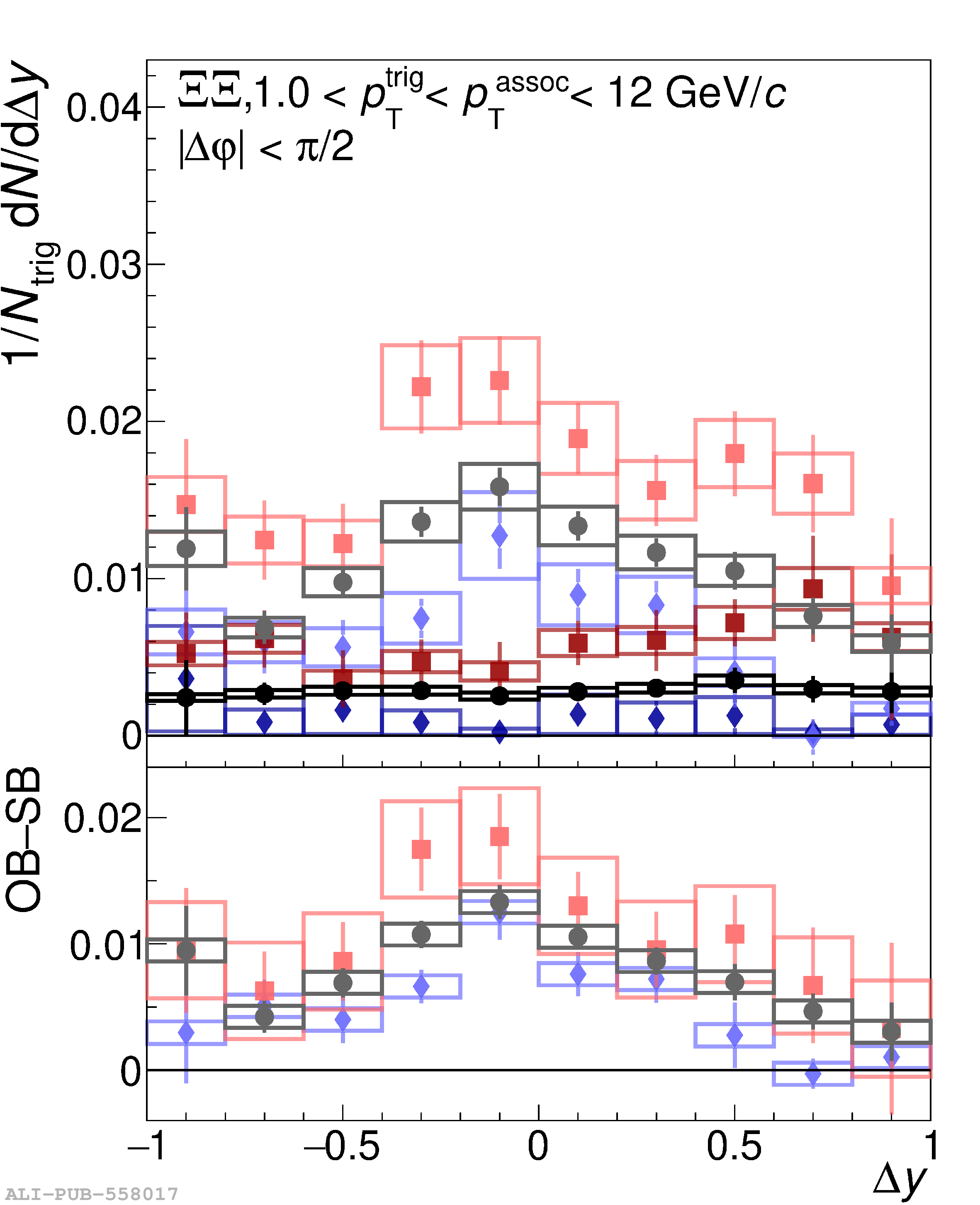 |
Figure 12
The integrated OS$-$SS near-side yields (top) and near-side RMS widths in $\Delta y$ (bottom) are shown for $\Xi\pi$ (left) and $\Xi\mathrm{K}$ (right) correlations as a function of multiplicity. Statistical and systematic uncertainties are represented by bars and boxes, respectively. The ALICE data are compared with the following models: PYTHIA 8 Monash tune (blue), PYTHIA 8 with junctions enabled (green), PYTHIA 8 with junctions and ropes (yellow), EPOS-LHC (red), and HERWIG 7 (pink). The statistical uncertainties on the model predictions, denoted by vertical bars, are smaller than the marker sizes in most cases. |   |
Figure 13
The integrated OB$-$SB near-side yields (top) and near-side RMS widths in $\Delta y$ (bottom) are shown for $\Xi\mathrm{p}$ (left) and $\Xi\Lambda$ (right) correlations as a function of multiplicity. Statistical and systematic uncertainties are represented by bars and boxes, respectively. The ALICE data are compared with the following models: PYTHIA 8 Monash tune (blue), PYTHIA 8 with junctions enabled (green), PYTHIA 8 with junctions and ropes (yellow), EPOS-LHC (red), and HERWIG 7 (pink). The statistical uncertainties on the model predictions, denoted by vertical bars, are smaller than the marker sizes in most cases. |  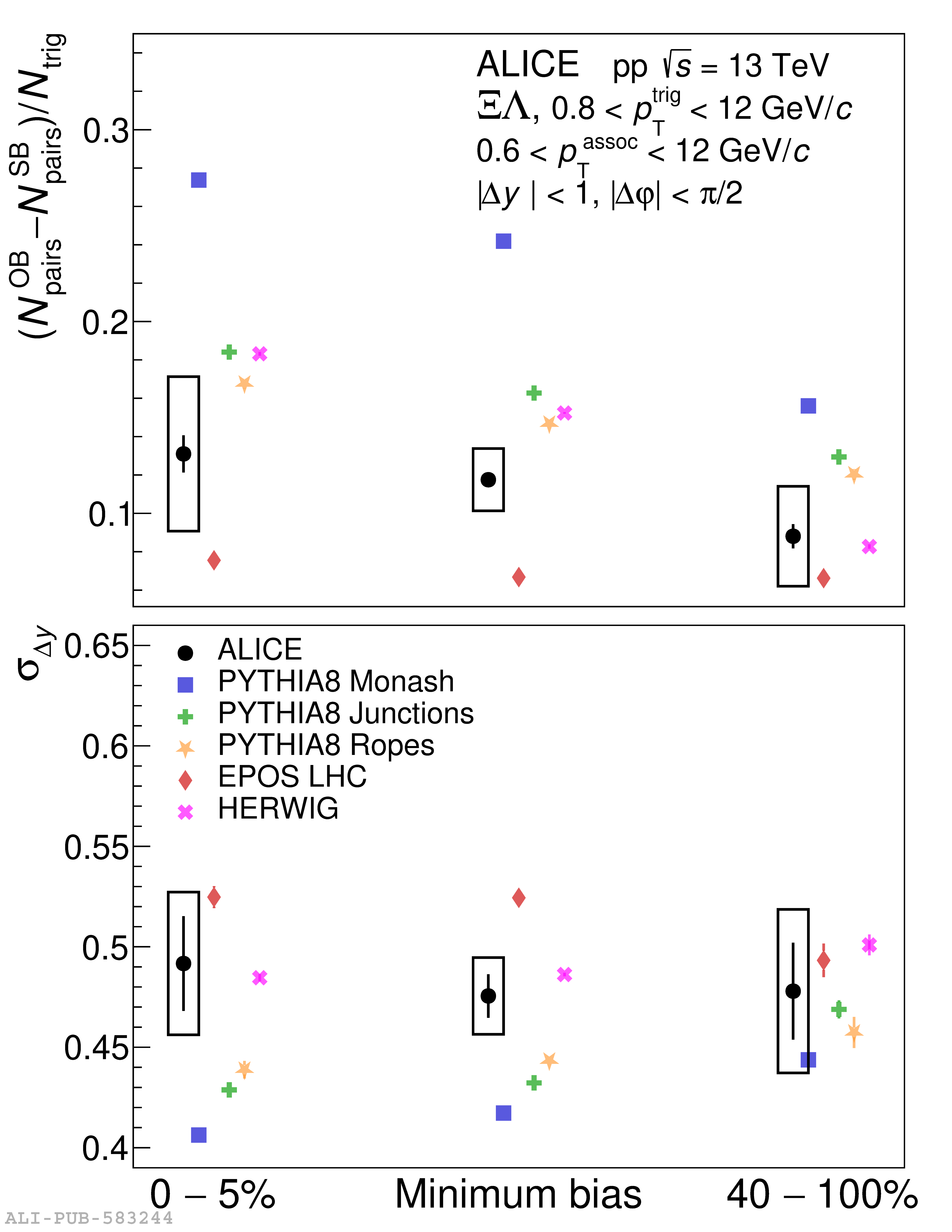 |
Figure 14
The integrated OB$-$SB near-side yields (top) and near-side RMS widths in $\Delta y$ (bottom) are shown for $\Xi\Xi$ correlations as a function of multiplicity. Statistical and systematic uncertainties are represented by bars and boxes, respectively. The ALICE data are compared with the following models: PYTHIA 8 Monash tune (blue), PYTHIA 8 with junctions enabled (green), PYTHIA 8 with junctions and ropes (yellow), EPOS-LHC (red), and HERWIG 7 (pink). The statistical uncertainties on the model predictions, denoted by vertical bars, are smaller than the marker sizes in most cases. | 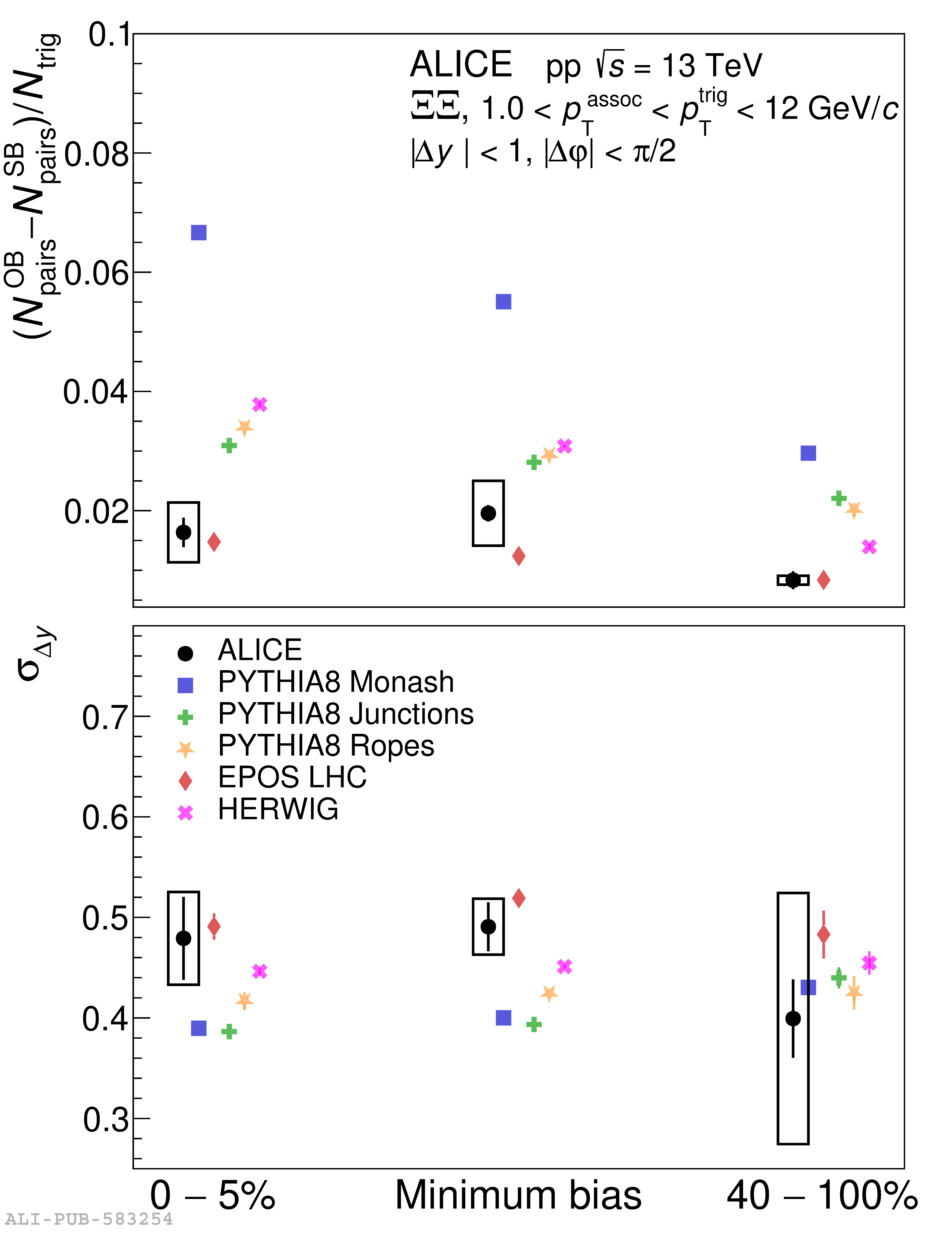 |