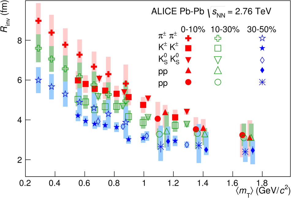
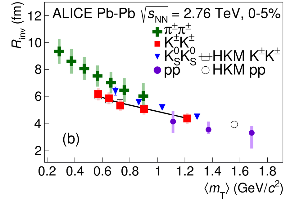
The size of the particle emission region in high-energy collisions can be deduced using the femtoscopic correlations of particle pairs at low relative momentum. Such correlations arise due to quantum statistics and Coulomb and strong final state interactions. In this paper, results are presented from femtoscopic analyses of $\pi^{\pm}\pi^{\pm}$, ${\rm K}^{\pm}{\rm K}^{\pm}$, ${\rm K}^{0}_S{\rm K}^{0}_S$, ${\rm pp}$, and ${\rm \overline{p}}{\rm \overline{p}}$ correlations from Pb-Pb collisions at $\sqrt{s_{\mathrm {NN}}}=2.76$ TeV by the ALICE experiment at the LHC. One-dimensional radii of the system are extracted from correlation functions in terms of the invariant momentum difference of the pair. The comparison of the measured radii with the predictions from a hydrokinetic model is discussed. The pion and kaon source radii display a monotonic decrease with increasing average pair transverse mass $m_{\rm T}$ which is consistent with hydrodynamic model predictions for central collisions. The kaon and proton source sizes can be reasonably described by approximate $m_{\rm T}$-scaling.
Phys. Rev. C 92 (2015) 054908
HEP Data
e-Print: arXiv:1506.07884 | PDF | inSPIRE
CERN-PH-EP-2015-106

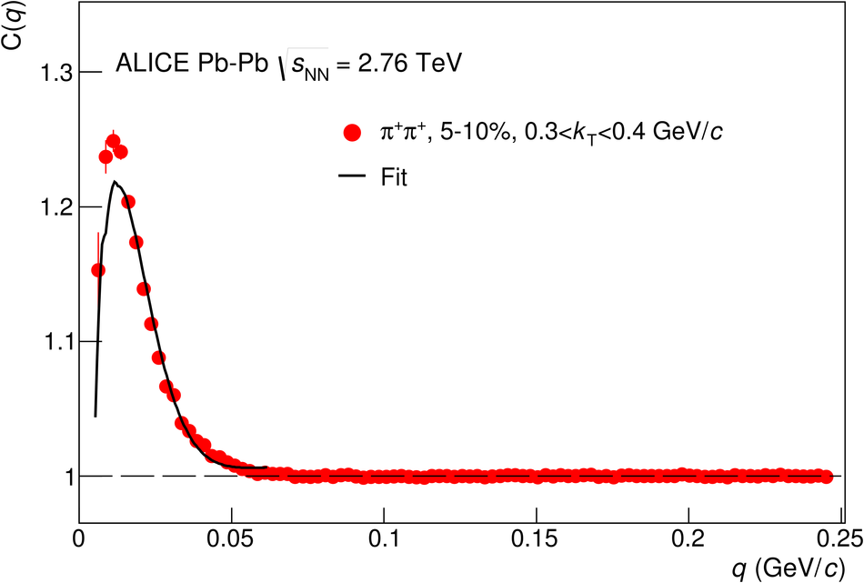
Figure 4
Example correlation function with fit for $\rm K^{\pm}\rm K^{\pm}$ for centrality 0-10% and $\left < k_{\rm T} \right > = 0.35$ GeV/$c$. Systematic uncertainties (boxes) are shown; statistical uncertainties are within the data markers. The main sources of systematic uncertainty are the momentum resolution correction and PID selection. |  |
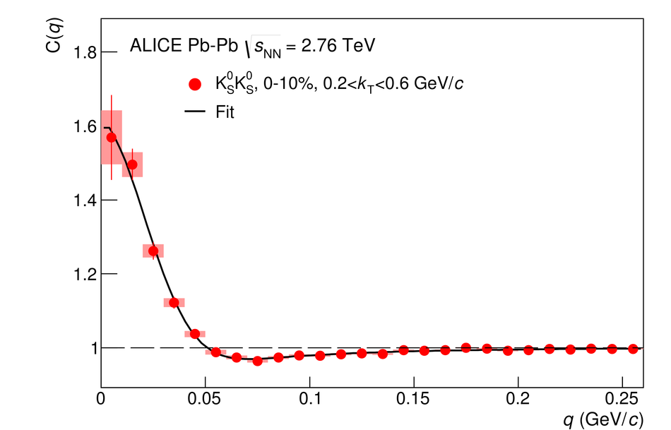
Figure 6
Example correlation function with fit for $\overline{\rm p}\overline{\rm p}$ for centrality 0-10% and $\left < k_{\rm T} \right > = 1.0$ GeV/$c$. Statistical (thin lines) and systematic (boxes) uncertainties are shown. The main source of systematic uncertainty is the variation of two-track cuts. | 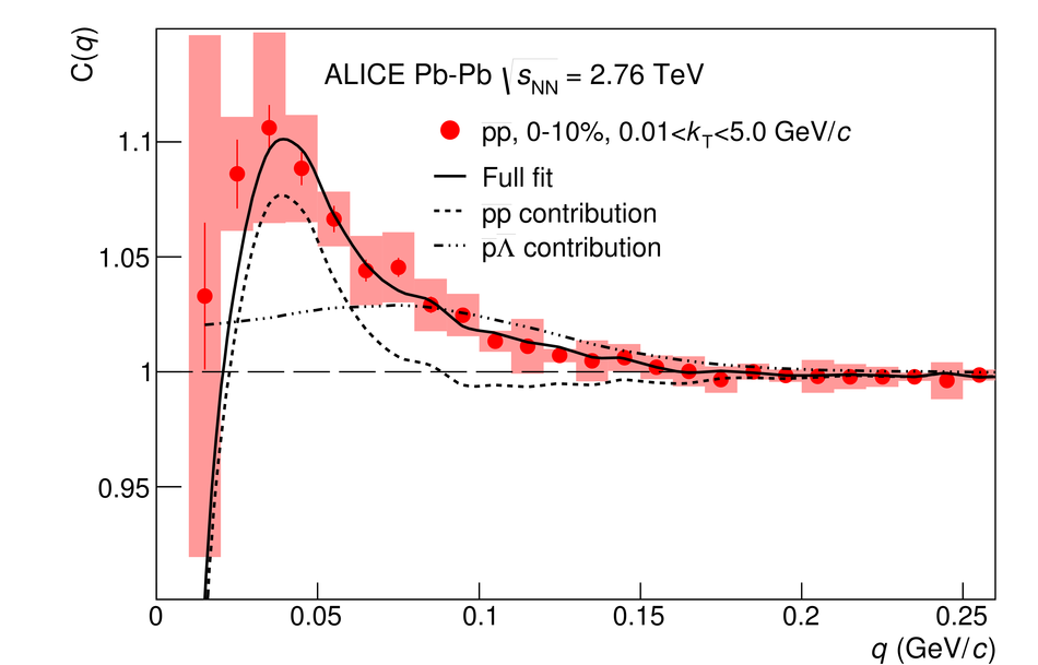 |
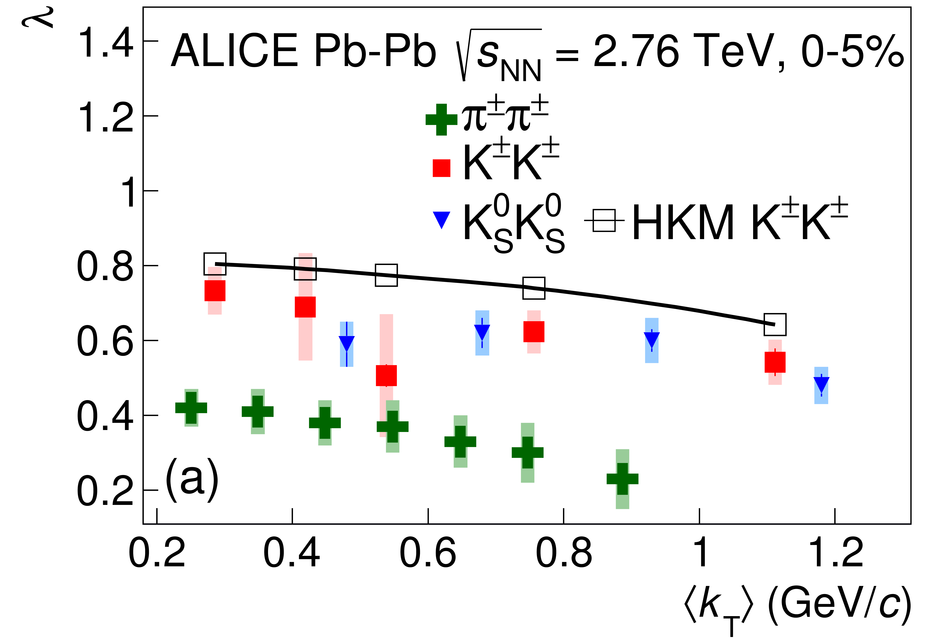
Figure 7
$\lambda$ parameters ($\lambda_{\rm {p}\rm {p}}+\lambda_{\rm {p}\Lambda}$ in case of (anti)proton pairs) vs. $m_{\rm T}$ for the three centralities considered for $\pi^{\pm}\pi^{\pm}$, $\rm K^{\pm}\rm K^{\pm}$,$\Kzs\Kzs$, $\rm {p}\rm {p}$, and $\overline{\rm p}\overline{\rm p}$. Statistical (thin lines) and systematic (boxes) uncertainties are shown. The $m_{\rm T}$ values for different centrality intervals are slightlyoffset for clarity. | 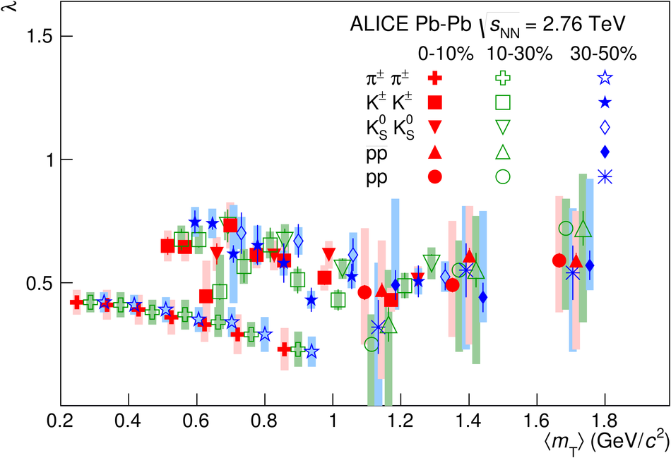 |