The jet angularities are a class of jet substructure observables which characterize the angular and momentum distribution of particles within jets. These observables are sensitive to momentum scales ranging from perturbative hard scatterings to nonperturbative fragmentation into final-state hadrons. We report measurements of several groomed and ungroomed jet angularities in pp collisions at $\sqrt{s}=5.02$ TeV with the ALICE detector. Jets are reconstructed using charged particle tracks at midrapidity ($|\eta| <~ 0.9$). The anti-$k_{\rm T}$ algorithm is used with jet resolution parameters $R=0.2$ and $R=0.4$ for several transverse momentum $p_{\rm T}^{\text{ch jet}}$ intervals in the 20$-$100 GeV/$c$ range. Using the jet grooming algorithm Soft Drop, the sensitivity to softer, wide-angle processes, as well as the underlying event, can be reduced in a way which is well-controlled in theoretical calculations. We report the ungroomed jet angularities, $\lambda_{\alpha}$, and groomed jet angularities, $\lambda_{\alpha\text{,g}}$, to investigate the interplay between perturbative and nonperturbative effects at low jet momenta. Various angular exponent parameters $\alpha = 1$, 1.5, 2, and 3 are used to systematically vary the sensitivity of the observable to collinear and soft radiation. Results are compared to analytical predictions at next-to-leading-logarithmic accuracy, which provide a generally good description of the data in the perturbative regime but exhibit discrepancies in the nonperturbative regime. Moreover, these measurements serve as a baseline for future ones in heavy-ion collisions by providing new insight into the interplay between perturbative and nonperturbative effects in the angular and momentum substructure of jets. They supply crucial guidance on the selection of jet resolution parameter, jet transverse momentum, and angular scaling variable for jet quenching studies.
JHEP 05 (2022) 061
HEP Data
e-Print: arXiv:2107.11303 | PDF | inSPIRE
CERN-EP-2021-145
Figure group
Figure 1
Comparison of ungroomed jet angularities \ang{} in \pp{}collisions for $R=0.4$ to MC predictions using PYTHIA8 and Herwig7, as described in the text. Four equally-sized \pTchjet{} intervals are shown, with edges ranging between 20 and 100 \GeVc{}. The distributions are normalized to unity. | 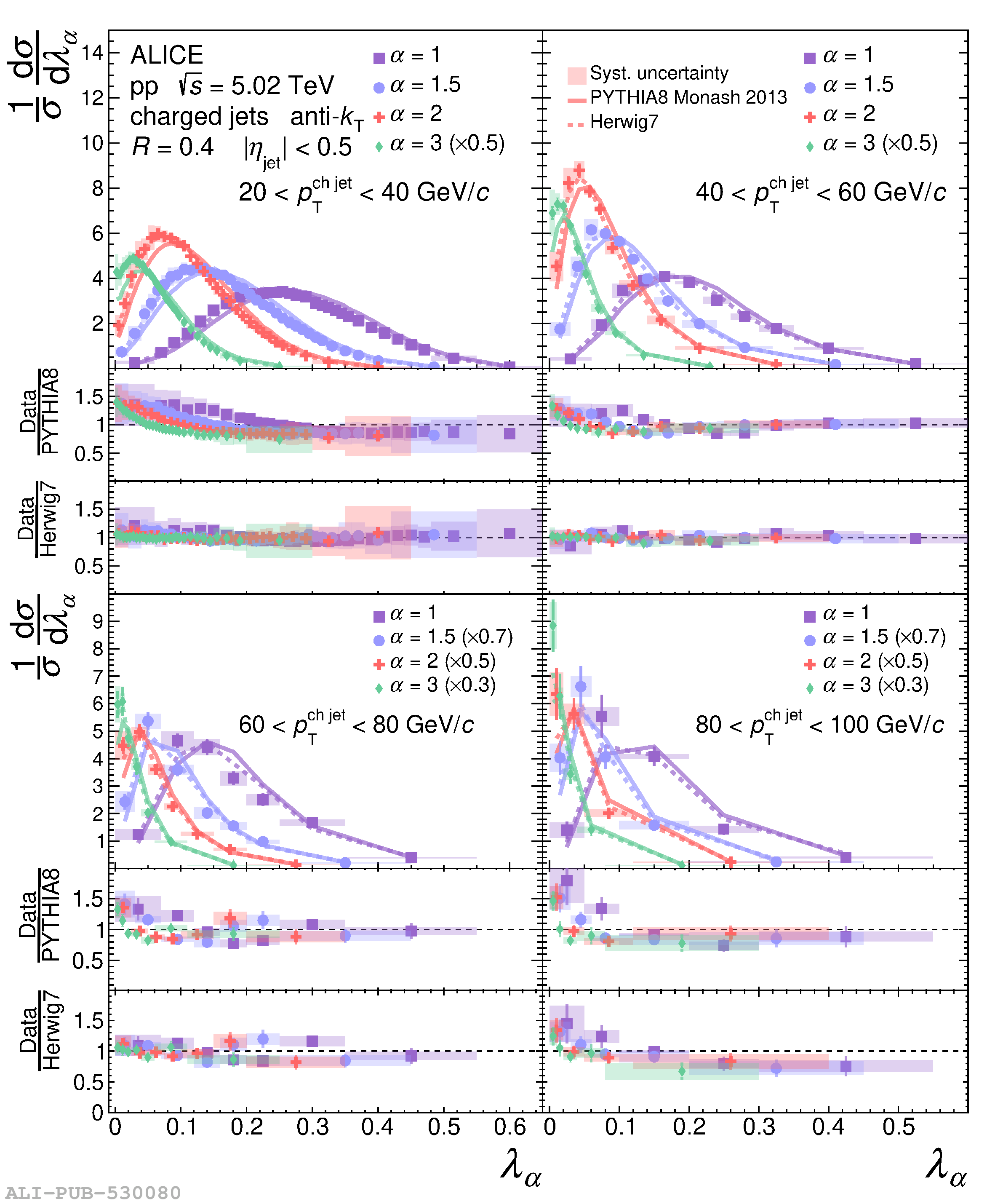 |
Figure 2
Comparison of ungroomed jet angularities \ang{} in \pp{}collisions for $R=0.2$ to MC predictions using PYTHIA8 and Herwig7, as described in the text. Four equally-sized \pTchjet{} intervals are shown, with edges ranging between 20 and 100 \GeVc{}. The distributions are normalized to unity. | 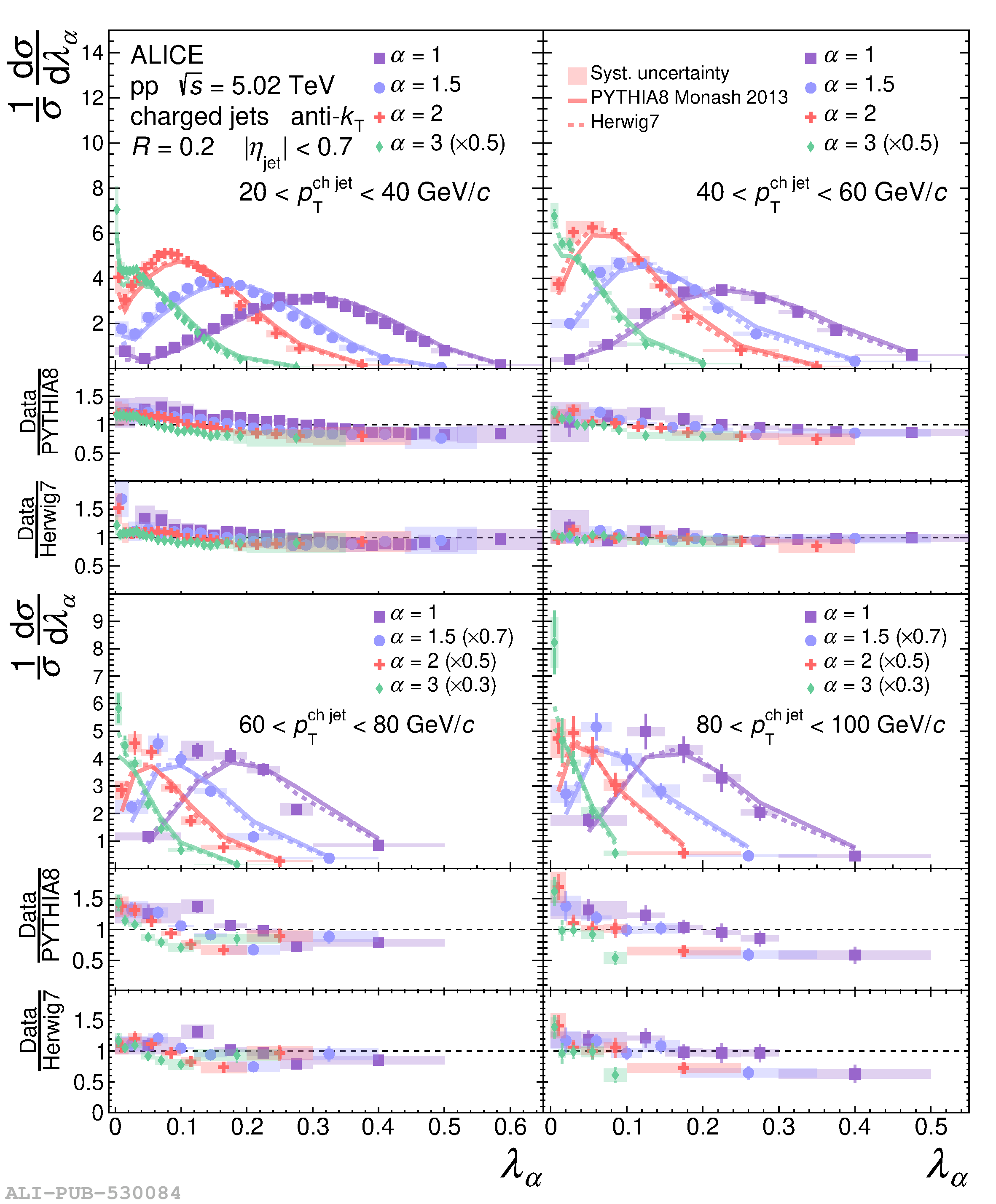 |
Figure 3
Comparison of groomed jet angularities \angsd{} in \pp{}collisions for $R=0.4$ to MC predictions using PYTHIA8 and Herwig7, as described in the text. Four equally-sized \pTchjet{} intervals are shown between 20 and 100 \GeVc{}. The distributions arenormalized to the groomed jet tagging fraction. | 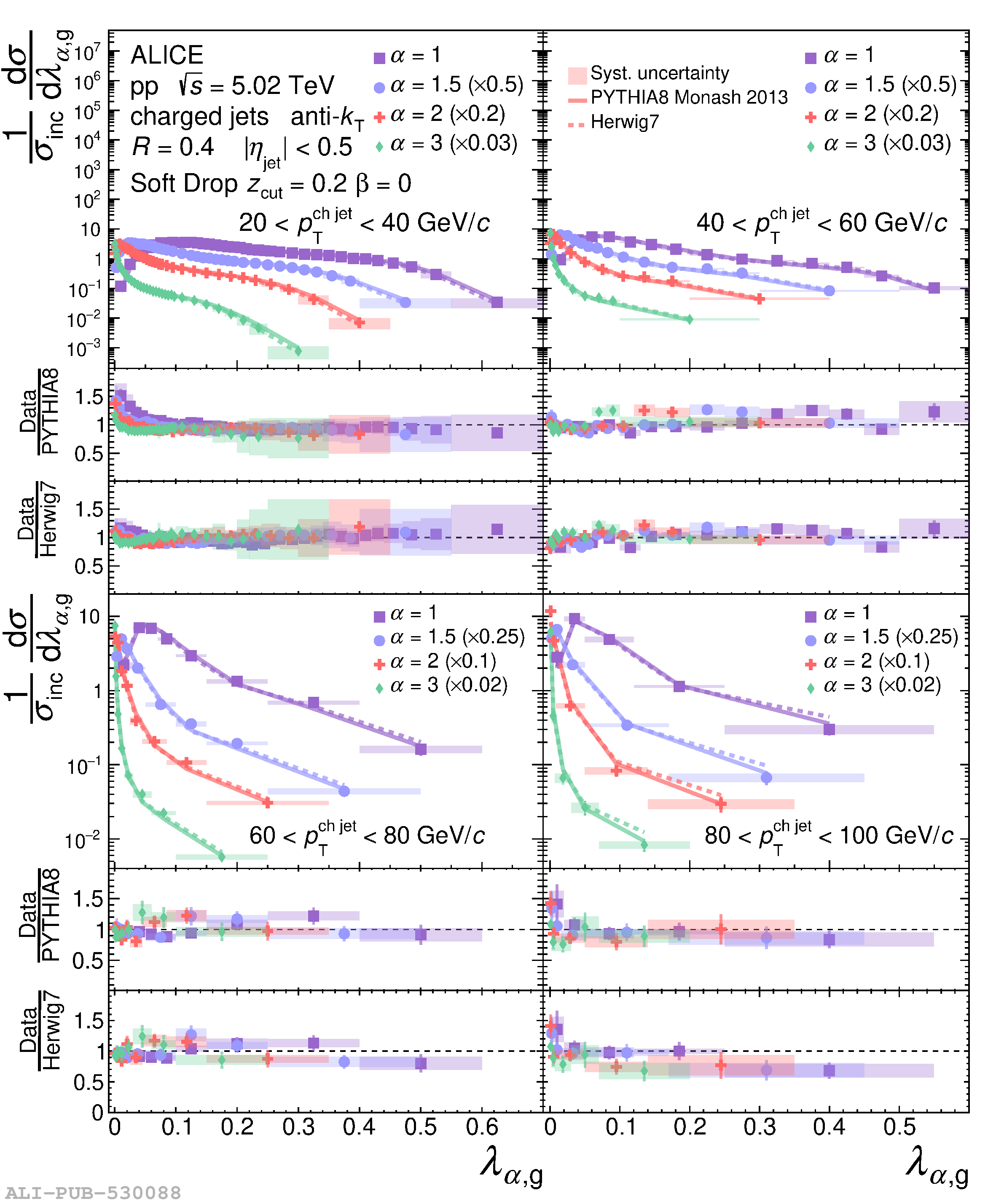 |
Figure 4
Comparison of groomed jet angularities \angsd{} in \pp{}collisions for $R=0.2$ to MC predictions using PYTHIA8 and Herwig7, as described in the text. Four equally-sized \pTchjet{} intervals are shown between 20 and 100 \GeVc{}. The distributions arenormalized to the groomed jet tagging fraction. | 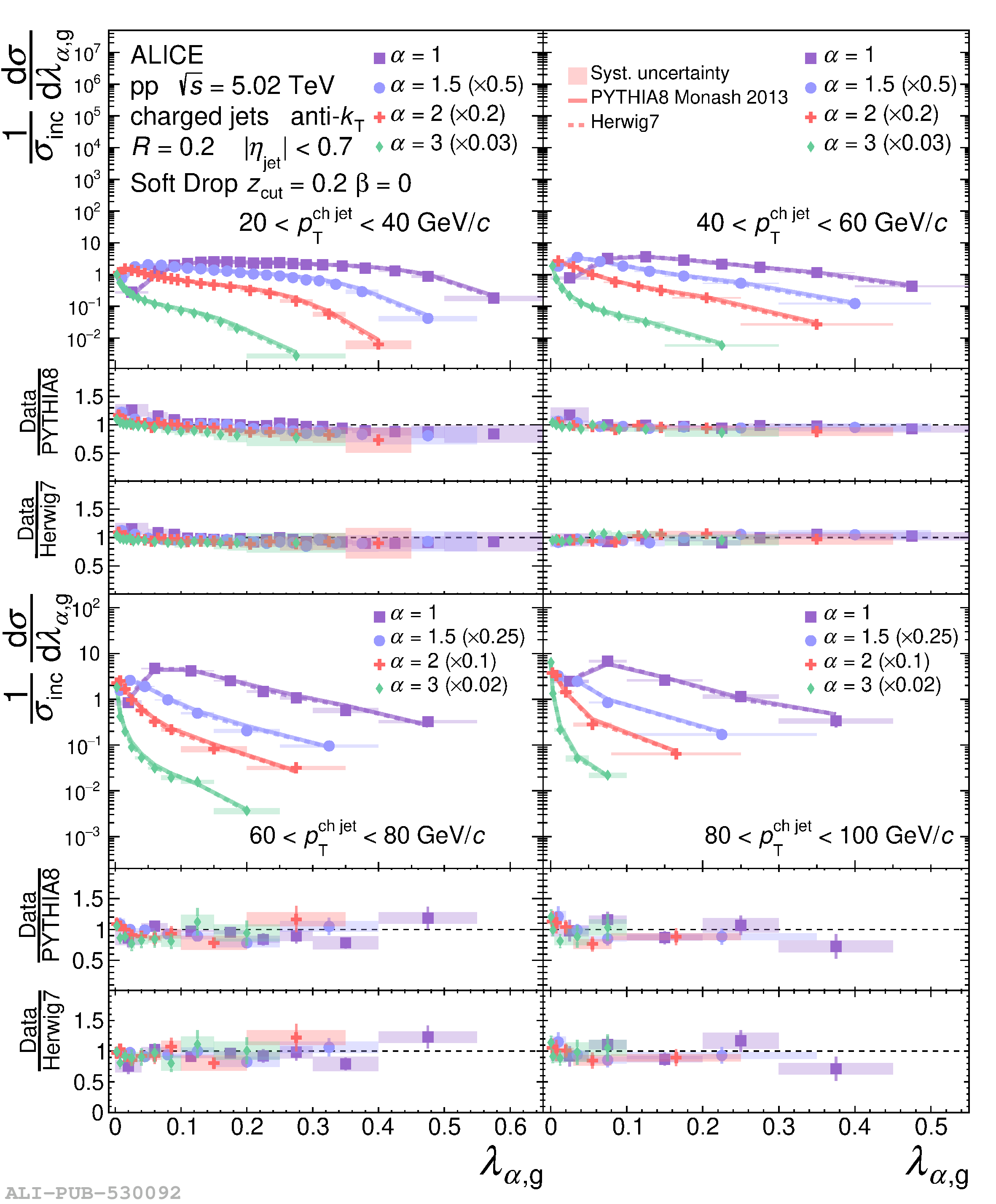 |
Figure 5
Comparison of ungroomed jet angularities \ang{} in \pp{}collisions for $R=0.2$ (top) and $R=0.4$ (bottom) to analyticalNLL$^\prime$ predictions with MC hadronization corrections in therange $60 < \pTchjet{} < 80$ \GeVc{}. The distributions arenormalized such that the integral of the perturbative region definedby $\ang > \angNP{}$ (to the right of the dashed vertical line)is unity. Divided bins are placed into the left (NP) region. | 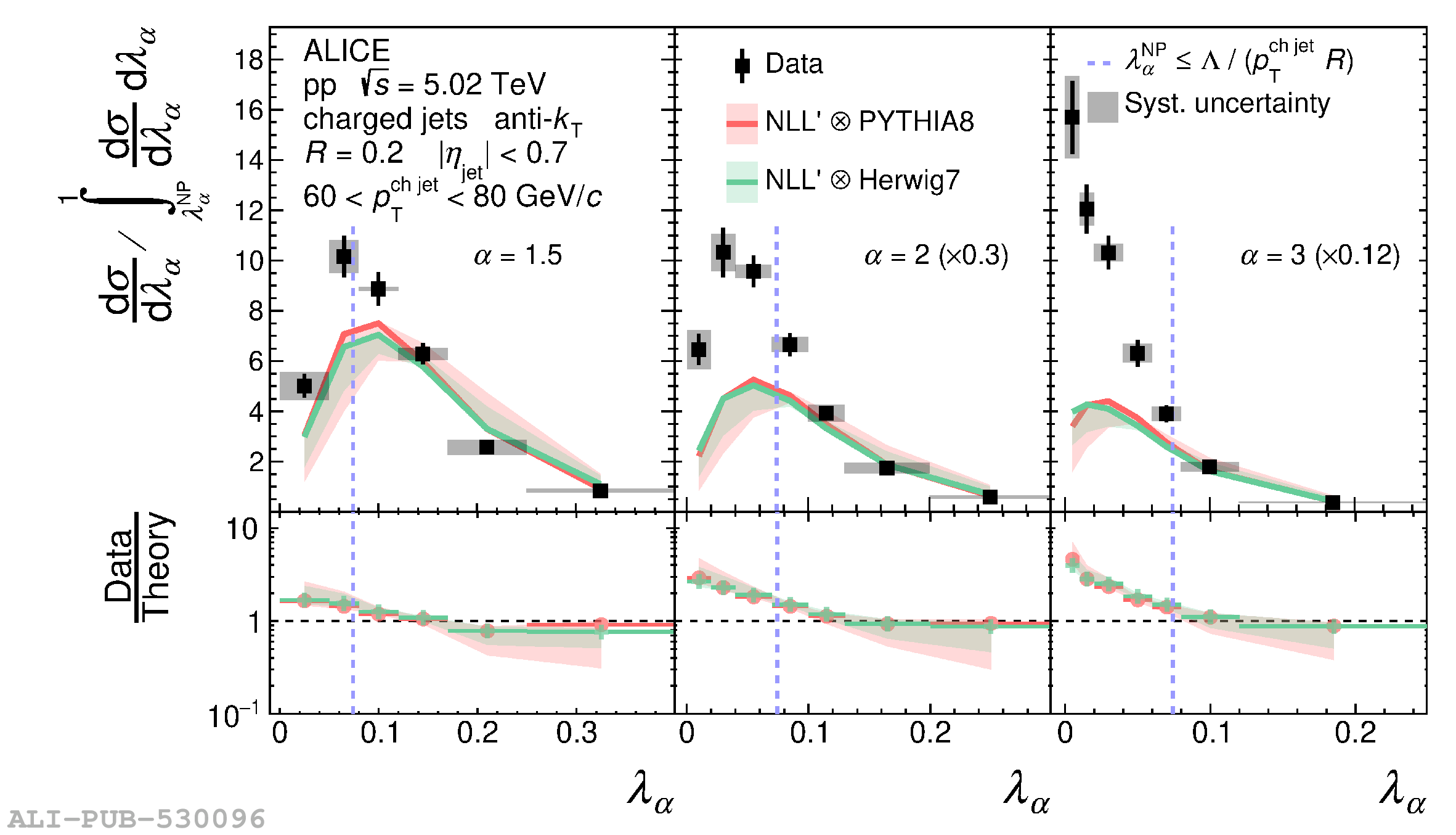  |
Figure 6
Comparison of groomed jet angularities \angsd{} in \pp{}collisions for $R=0.2$ (top) and $R=0.4$ (bottom) to analyticalNLL$^\prime$ predictions with MC hadronization corrections in therange $60 < \pTchjet{} < 80$ \GeVc{}. The distributions arenormalized such that the integral of the perturbative region definedby $\angsd > \angsdNP{}$ (to the right of the dashed vertical line)is unity. Divided bins are placed into the left (NP) region. | 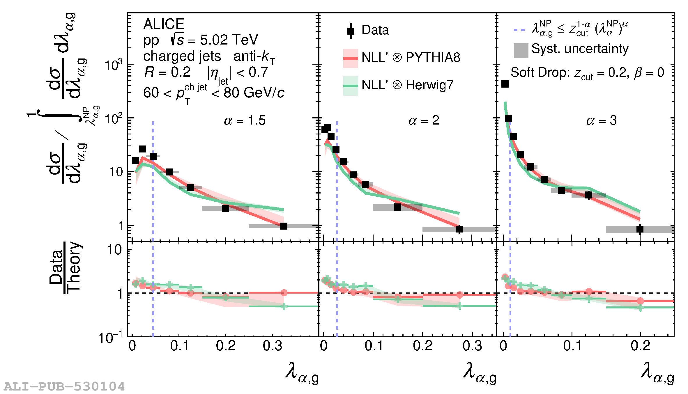 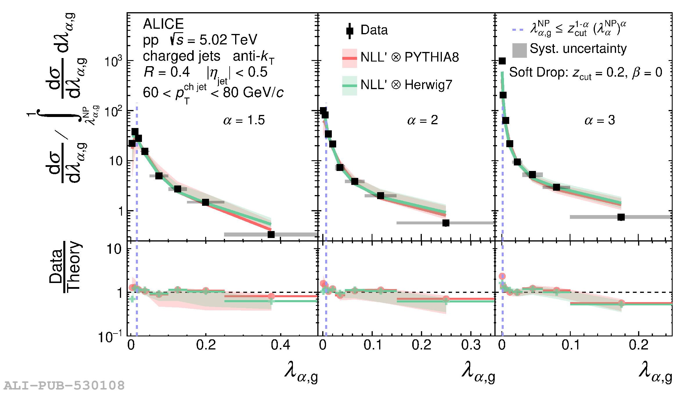 |
Figure 7
Comparison of ungroomed jet angularities \ang{} in \pp{}collisions for $R=0.2$ (top) and $R=0.4$ (bottom) to analyticalNLL$^\prime$ predictions using $F(k)$ convolution in therange $60 < \pTchjet{} < 80$ \GeVc{}. The distributions arenormalized such that the integral of the perturbative region definedby $\ang > \angNP{}$ (to the right of the dashed vertical line)is unity. Divided bins are placed into the left (NP) region. | 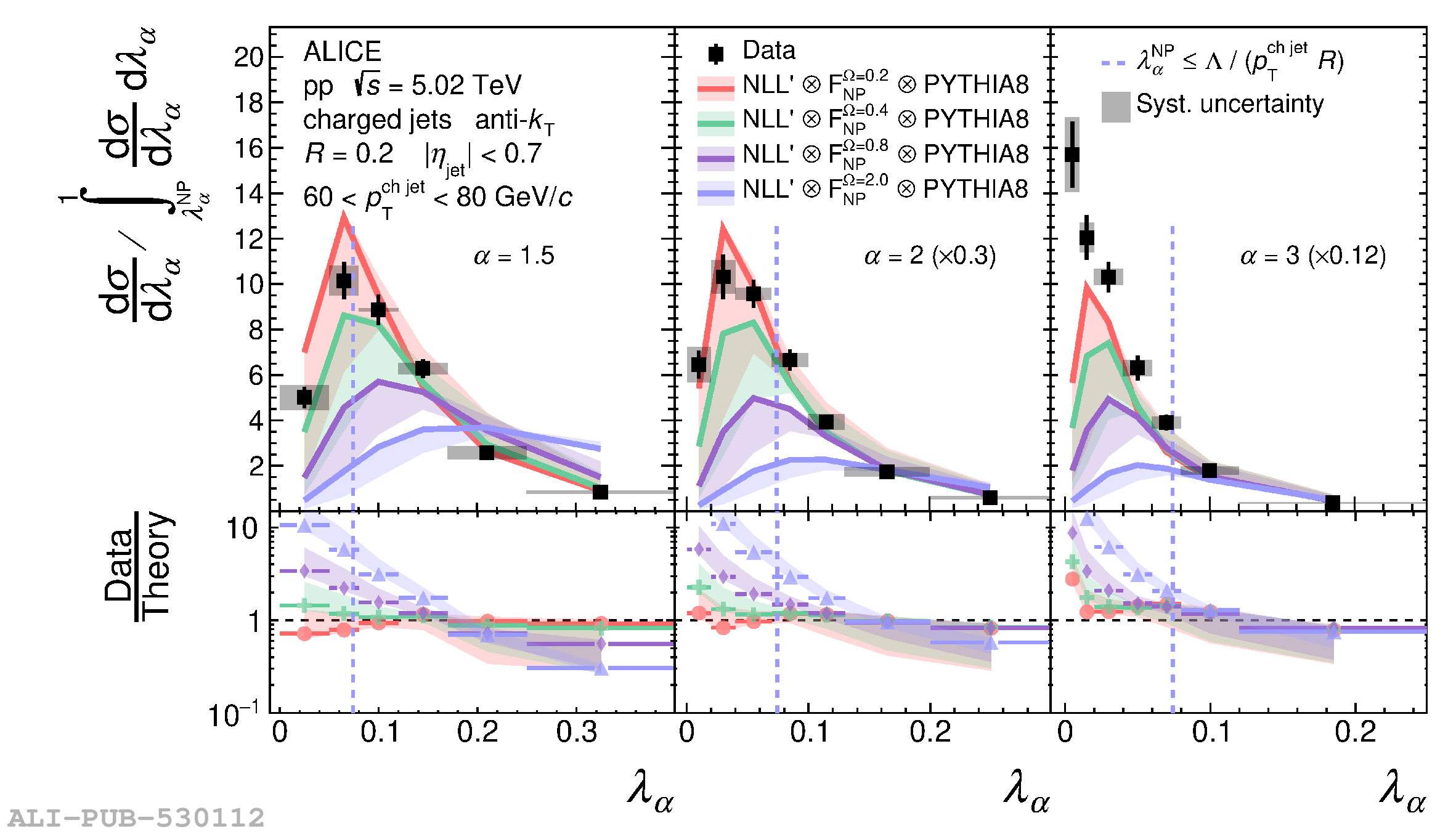 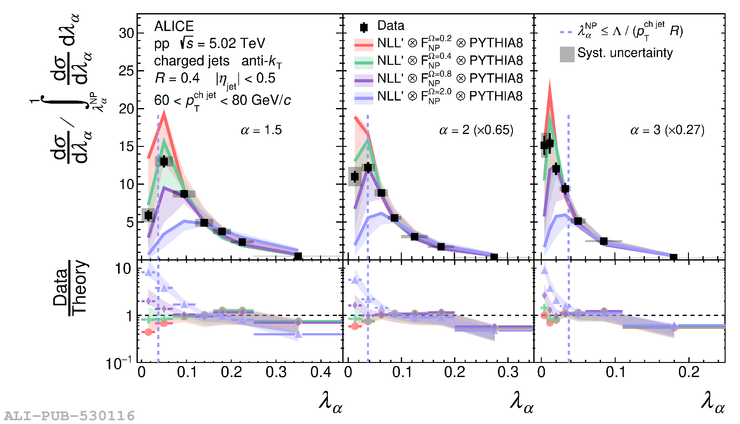 |
Figure 8
Comparison of groomed jet angularities \angsd{} in \pp{}collisions for $R=0.2$ (top) and $R=0.4$ (bottom) to analyticalNLL$^\prime$ predictions using $F(k)$ convolution in therange $60 < \pTchjet{} < 80$ \GeVc{}. The distributions arenormalized such that the integral of the perturbative region definedby $\angsd > \angsdNP{}$ (to the right of the dashed vertical line)is unity. Divided bins are placed into the left (NP) region. | 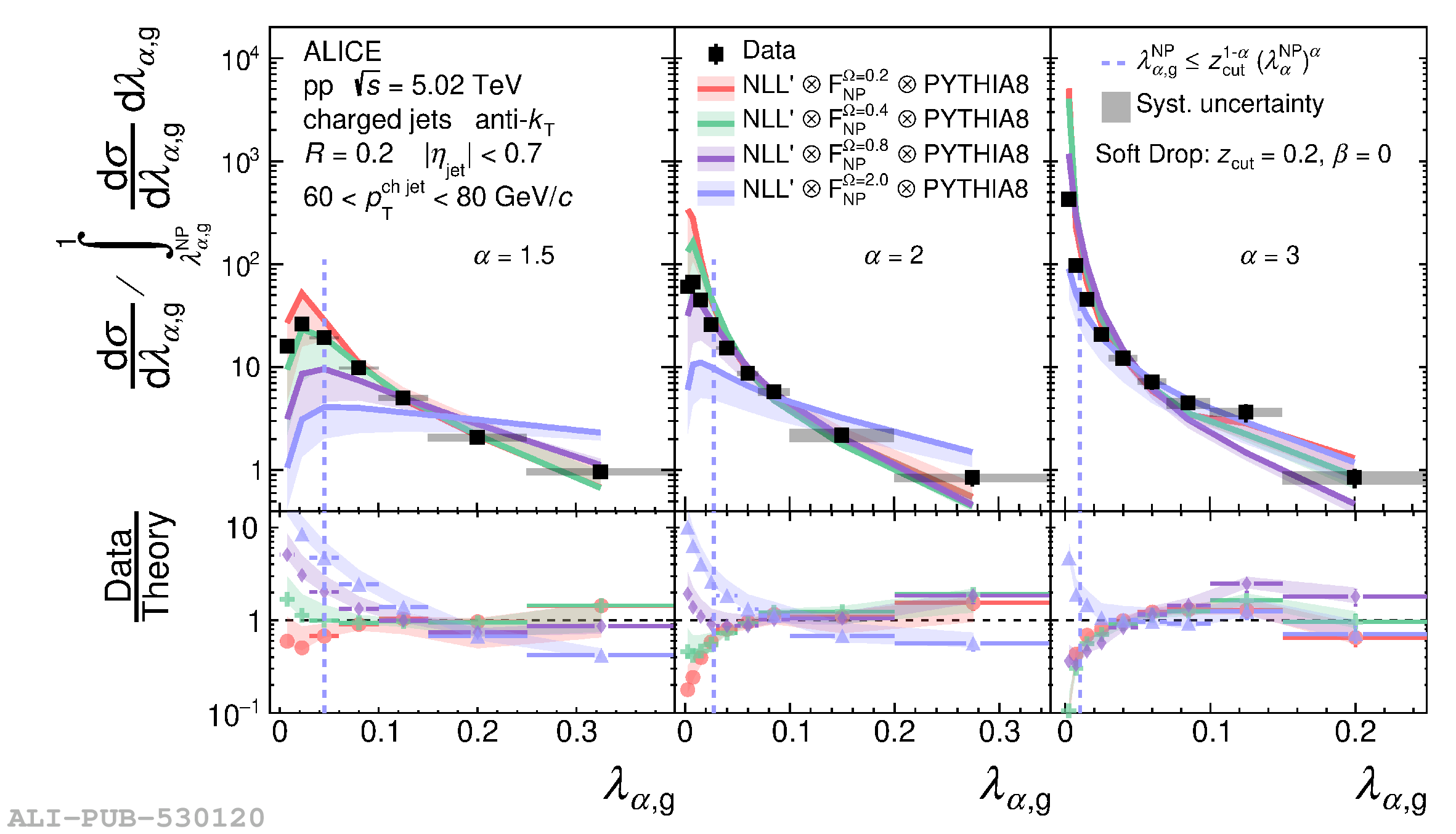  |
Figure A.1
Comparison of ungroomed jet angularities \ang{} in \pp{}collisions for $R=0.2$ (top) and $R=0.4$ (bottom) to analyticalNLL$^\prime$ predictions with MC hadronization corrections in therange $80 < \pTchjet{} < 100$ \GeVc{}. The distributions arenormalized such that the integral of the perturbative region definedby $\ang > \angNP{}$ (to the right of the dashed vertical line)is unity. Divided bins are placed into the left (NP) region. | 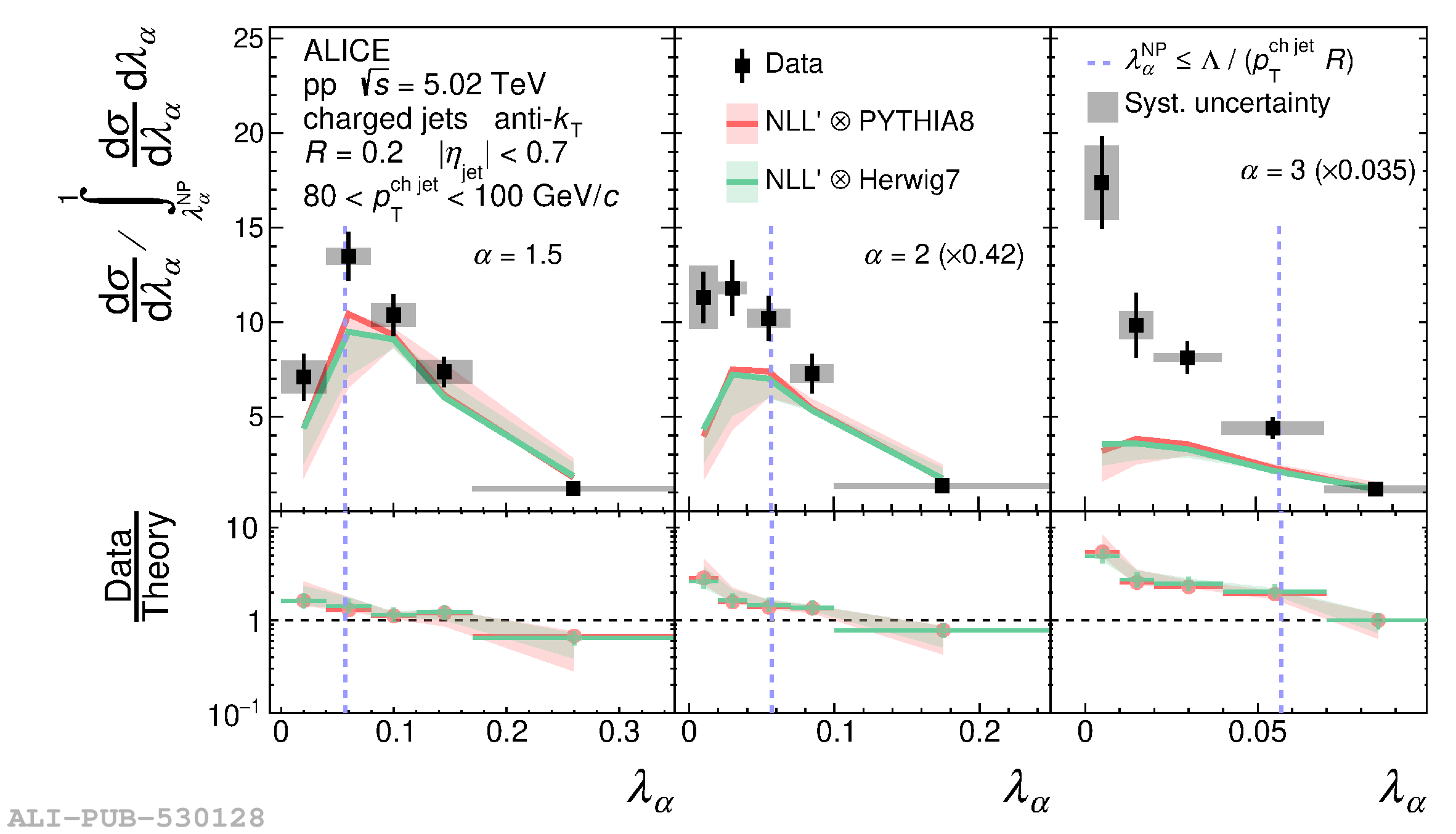 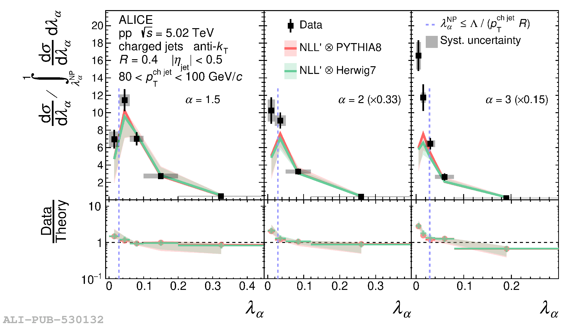 |
Figure A.2
Comparison of groomed jet angularities \angsd{} in \pp{}collisions for $R=0.2$ (top) and $R=0.4$ (bottom) to analyticalNLL$^\prime$ predictions with MC hadronization corrections in therange $80 < \pTchjet{} < 100$ \GeVc{}. The distributions arenormalized such that the integral of the perturbative region definedby $\angsd > \angsdNP{}$ (to the right of the dashed vertical line)is unity. Divided bins are placed into the left (NP) region. | 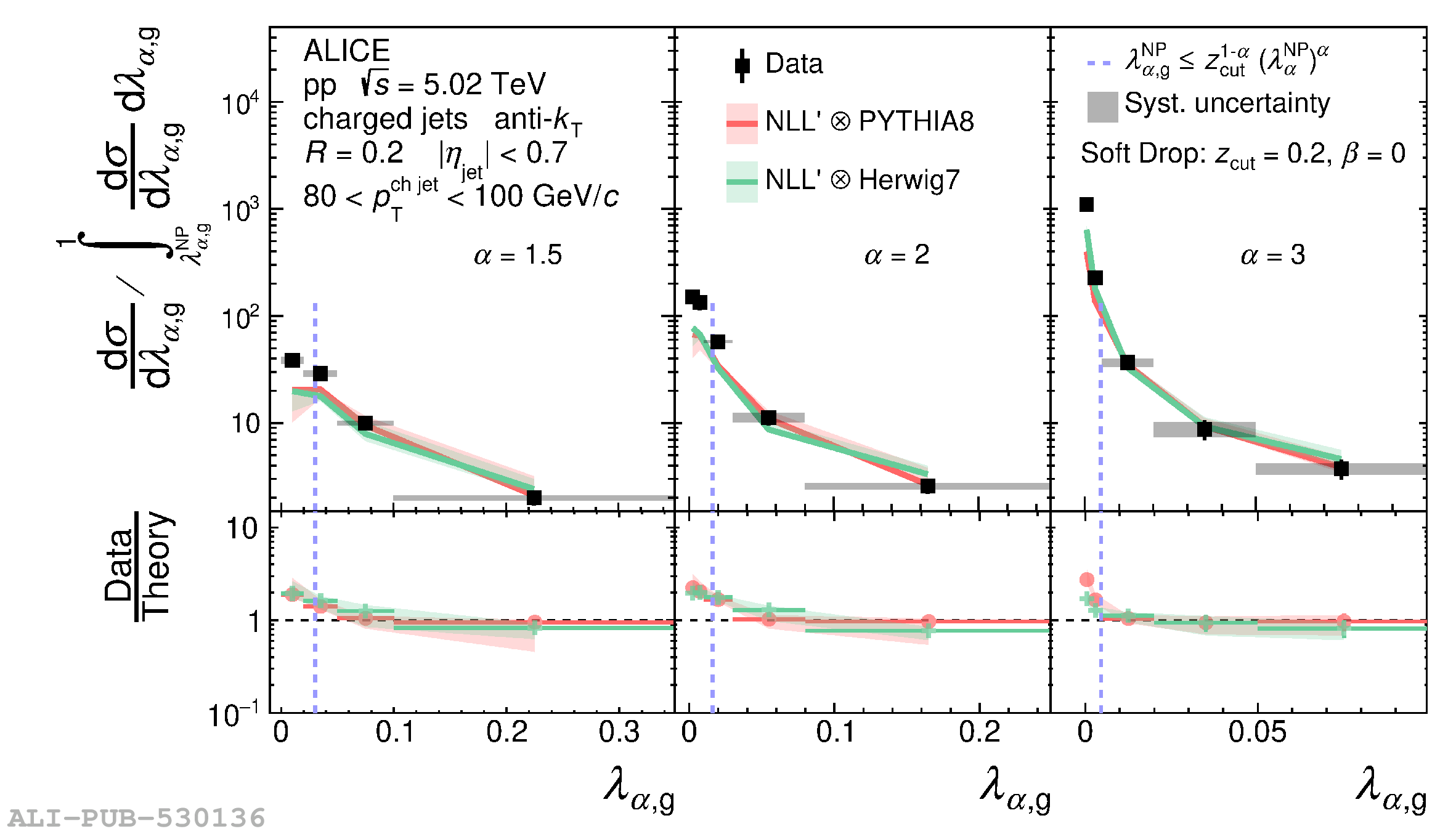  |
Figure A.3
Comparison of ungroomed jet angularities \ang{} in \pp{}collisions for $R=0.2$ (top) and $R=0.4$ (bottom) to analyticalNLL$^\prime$ predictions using $F(k)$ convolution in therange $40 < \pTchjet{} < 60$ \GeVc{}. The distributions arenormalized such that the integral of the perturbative region definedby $\ang > \angNP{}$ (to the right of the dashed vertical line)is unity. Divided bins are placed into the left (NP) region. | 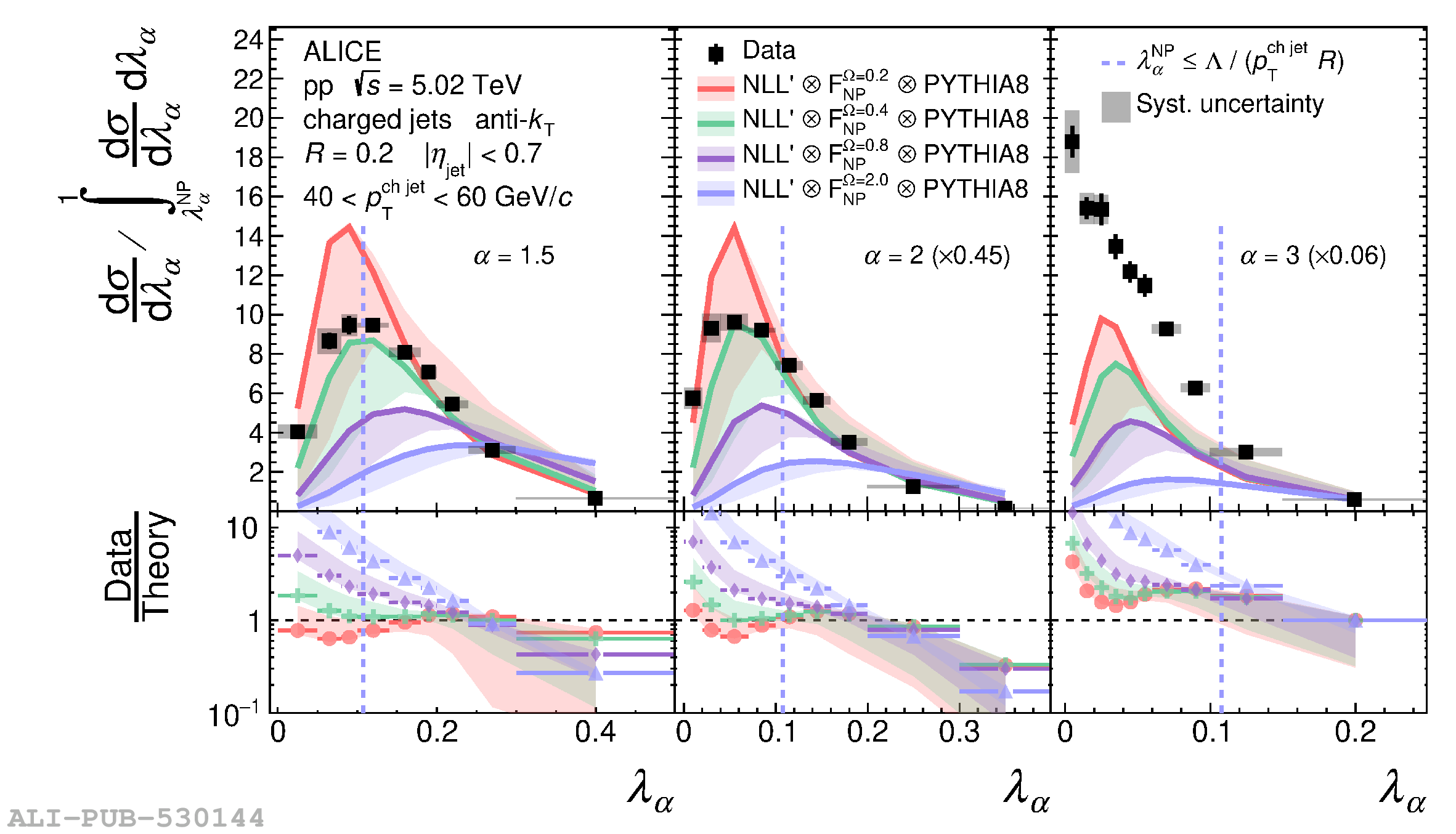 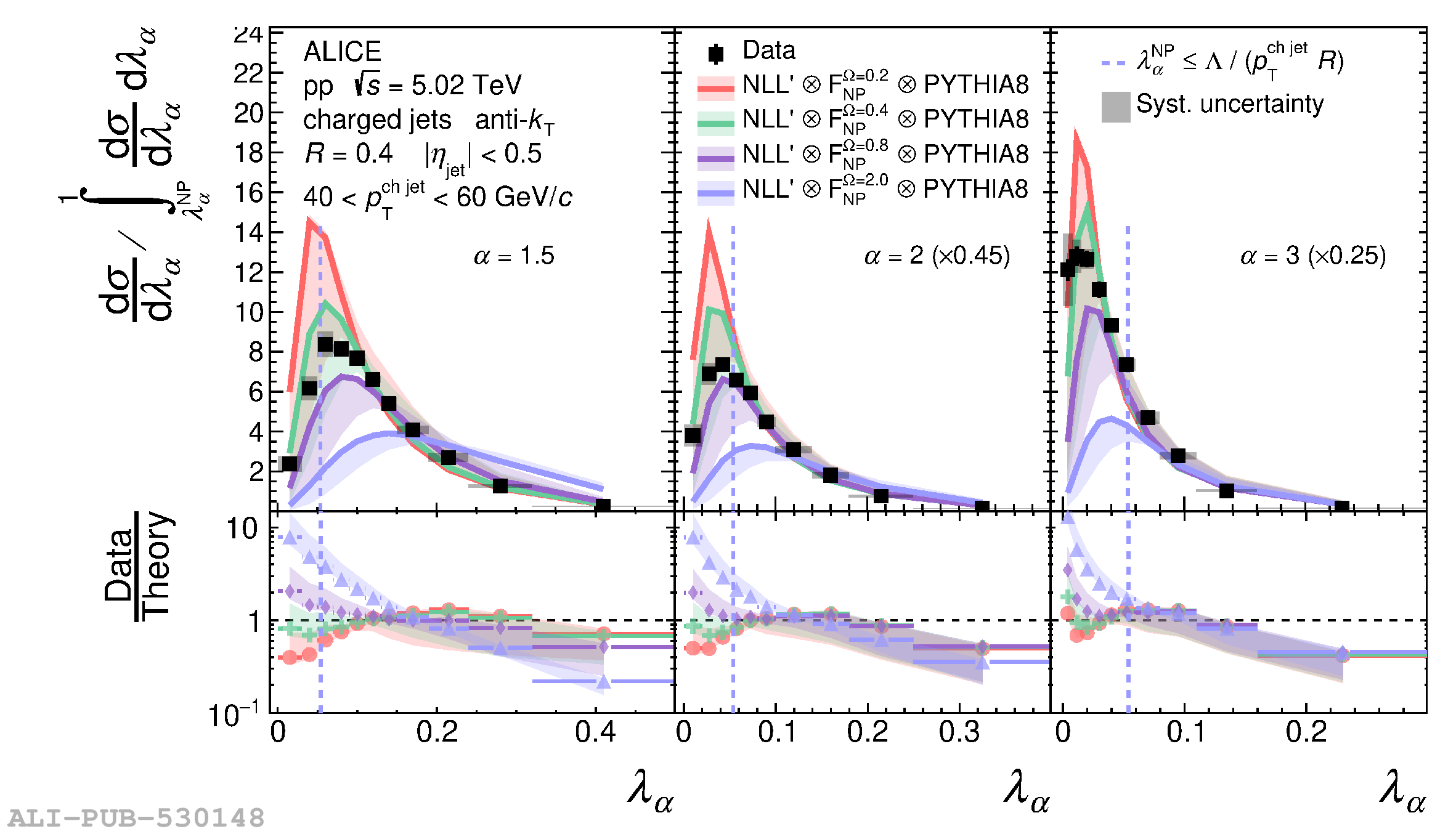 |
Figure A.4
Comparison of ungroomed jet angularities \ang{} in \pp{}collisions for $R=0.2$ (top) and $R=0.4$ (bottom) to analyticalNLL$^\prime$ predictions using $F(k)$ convolution in therange $80 < \pTchjet{} < 100$ \GeVc{}. The distributions arenormalized such that the integral of the perturbative region definedby $\ang > \angNP{}$ (to the right of the dashed vertical line)is unity. Divided bins are placed into the left (NP) region. | 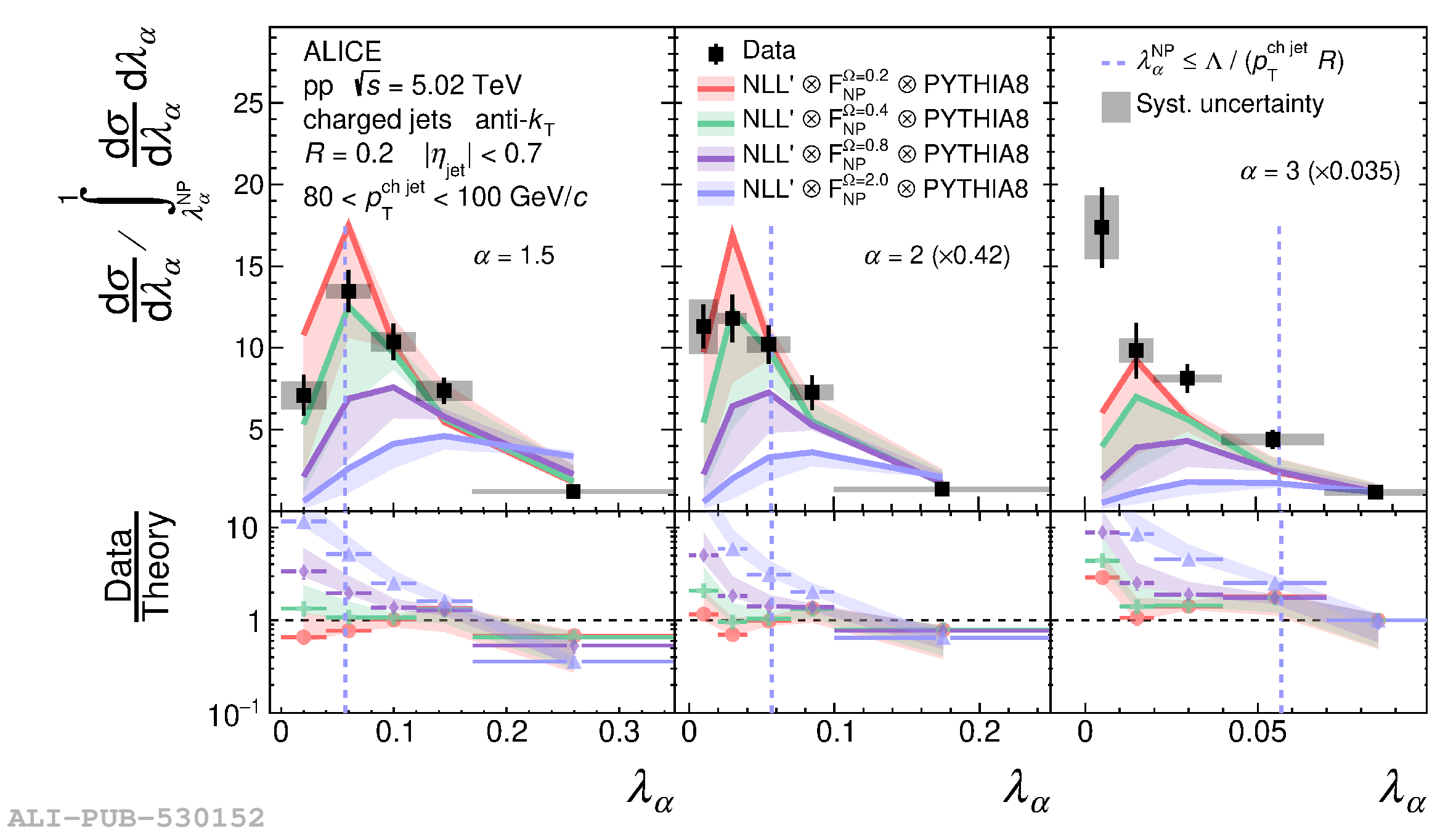 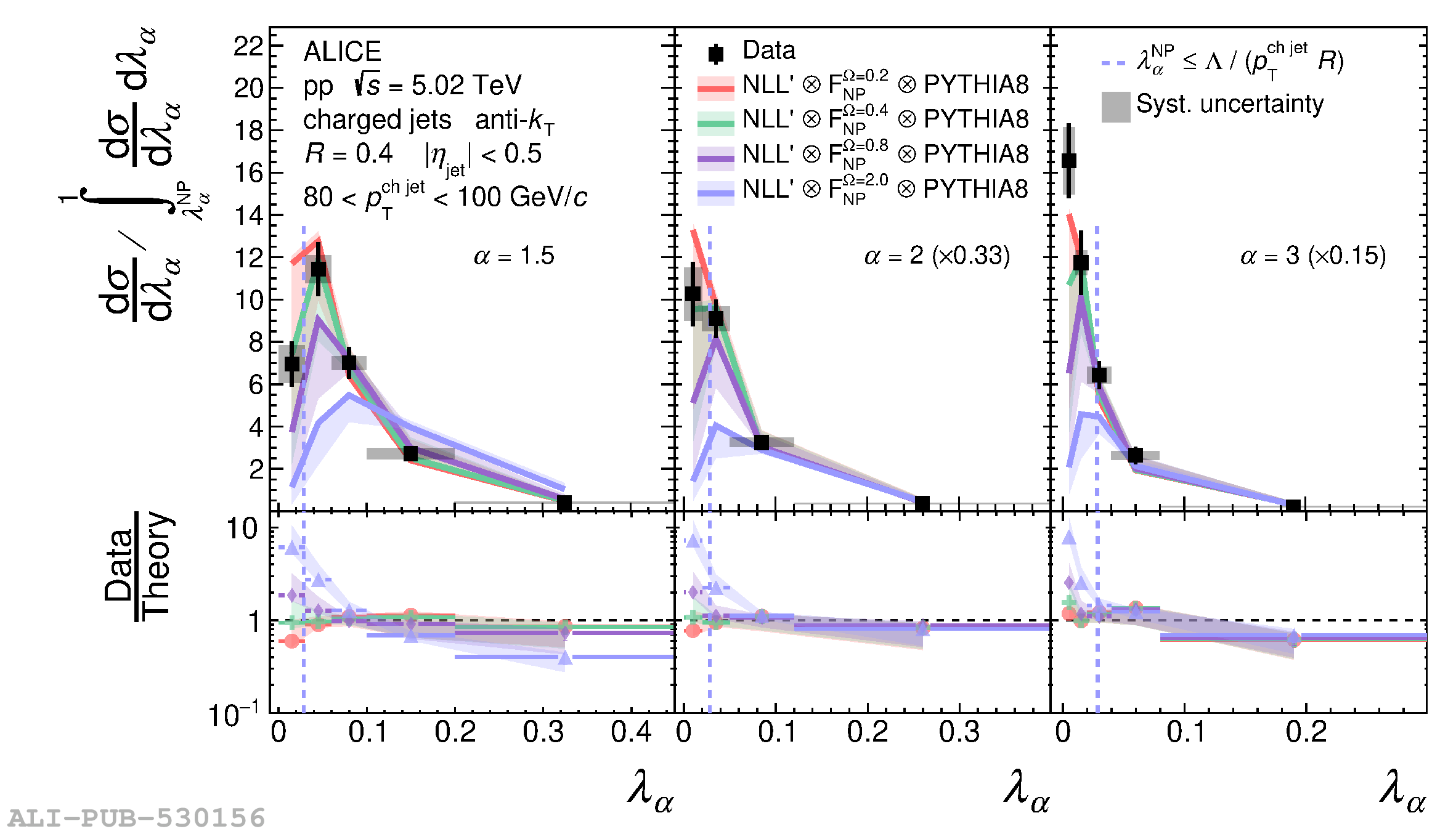 |
Figure A.5
Comparison of groomed jet angularities \angsd{} in \pp{}collisions for $R=0.2$ (top) and $R=0.4$ (bottom) to analyticalNLL$^\prime$ predictions using $F(k)$ convolution in therange $40 < \pTchjet{} < 60$ \GeVc{}. The distributions arenormalized such that the integral of the perturbative region definedby $\angsd > \angsdNP{}$ (to the right of the dashed vertical line)is unity. Divided bins are placed into the left (NP) region. | 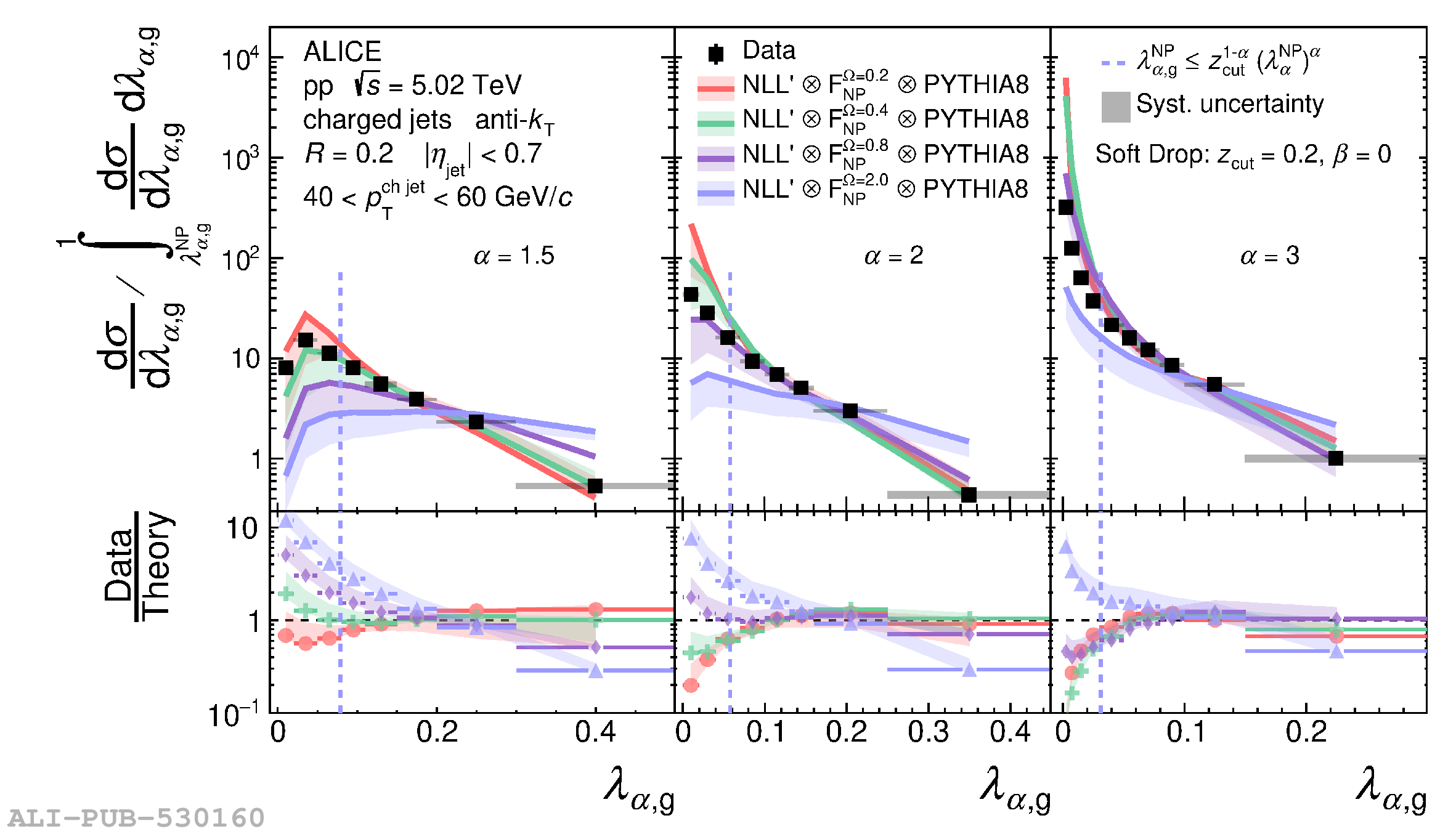 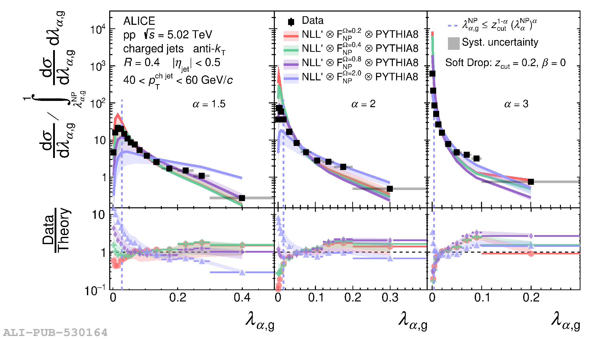 |
Figure A.6
Comparison of groomed jet angularities \angsd{} in \pp{}collisions for $R=0.2$ (top) and $R=0.4$ (bottom) to analyticalNLL$^\prime$ predictions using $F(k)$ convolution in therange $80 < \pTchjet{} < 100$ \GeVc{}. The distributions arenormalized such that the integral of the perturbative region definedby $\angsd > \angsdNP{}$ (to the right of the dashed vertical line)is unity. Divided bins are placed into the left (NP) region. | 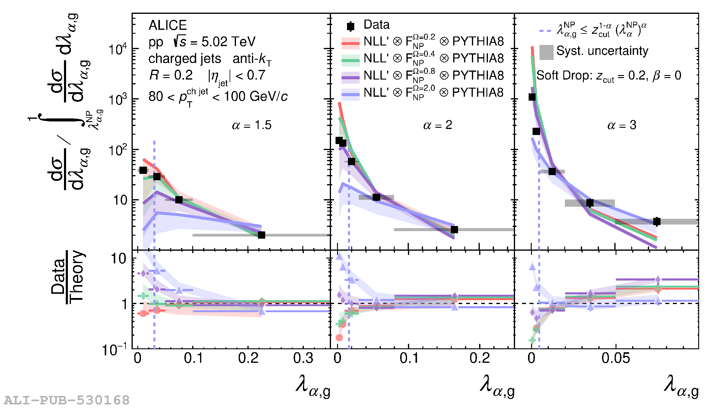 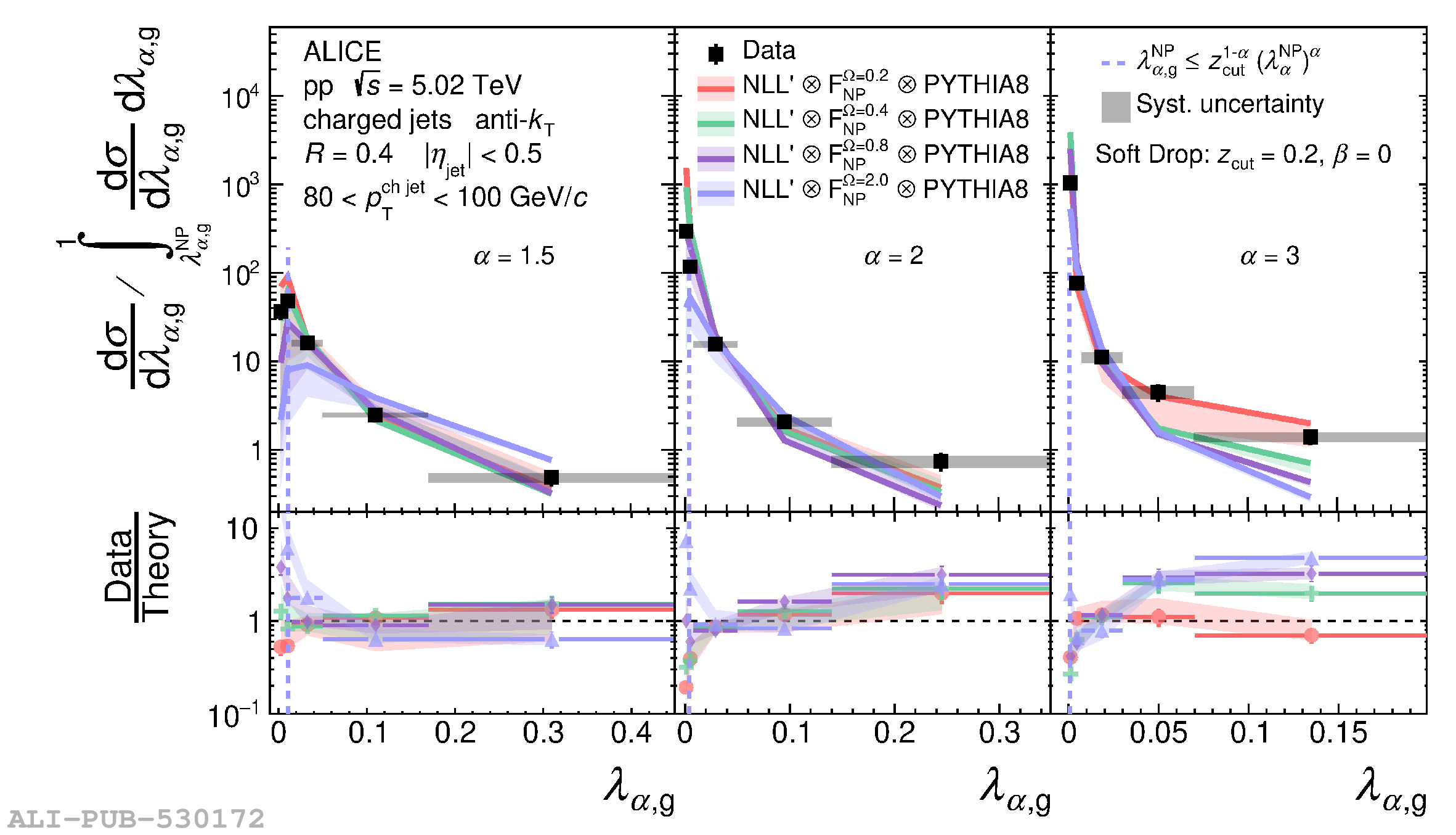 |